Proposals (Phase 1)

HSC queue mode proposals are submitted as Subaru Open Use programs, and all the basic policies of the Open Use apply to QM. For more information, see:

https://www.naoj.org/Observing/Visit/policy.html

A separate template is provided for the QM programs. The difference is that in QM the time is allocated in units of hours, where 1 h = 0.1 nights. PIs must first choose between classical and queue (recommended) modes, and estimate the number of required hours (on-source). The approximate dates of HSC runs, including the QM, will be communicated in the call for proposals (CfP). Gemini and Keck Telescope partners can apply through time exchange for QM observations. Time-critical programs are acceptable, and cadence observations are allowed only in the form of monitoring proposals (see Monitoring proposals). Some additional limitations may apply (see CfP for details). For the latest policy changes, please check the QM website, which is typically updated more often than the present document.

Proposal preparation

Additional targets

An important policy of the HSC operation, including QM, is the “no additional targets” rule, which means that all targets must be defined in Phase 1, and (with the exception of very special cases) no new targets will be allowed to be included in the program during the OB preparation and observation stages.

Some science programs may benefit from proposing more targets than may be possible to observe in the requested time, and defining the final sample after the acceptance and time allocation. During Phase 2 it is also possible to submit list of targets, where the total on-source time exceeds the allocation. Targets within one program can also be prioritized.

Some other restrictions apply to the selection of targets for HSC QM. See the “Clearly Prohibited Cases” in:

https://www.naoj.org/Observing/Visit/policy.html

Observing Constraints

Target selection depends on conditions at the time of observing, especially seeing, sky transparency, sky brightness (Moon phase) and distance to the Moon. If they change, schedule will accordingly be adjusted. The strictest of observing constraints must be defined in proposals for telscope time.

PIs must explicitly provide the following information:

Seeing
the maximum value of seeing, at which observations may be conducted, in arcsec.
Sky transparency
the lowest value of sky clearness and magnitude drop due to clouds, defined as a fraction between 0 (totally cloudy) and 1 (clear).
Moon phase/sky brightness
an acceptable brightness of the sky, due to illumination and elevation of the Moon - “dark” or “gray”. “Dark” is 0-3 days from the new moon or while the moon is below the horizon. “Gray” time is defined when the moon is above the horizon between 4 and 11 days from the new moon. HSC runs are not allocated in bright time.
Moon distance
the minimum separation from the Moon, at which angle targets can be observed, in degrees. Only distances larger than 30 deg are allowed (to avoid significant contamination by stray light). For “dark” time, it is 30 deg by default, and cannot be changed by PIs. For “gray” time, it must be set by PIs.
Time constraints
a window of time in which observations are to be conducted. There are no particular limits for its length, and multiple windows are allowed. A number of targets can be in a window, or it can be one target in a number of windows. Note that the more relaxed windows are, the higher the chances of OBs being executed.

NB Observing constraints in proposals must be the strictest ones.: seeing (upper limit), transparency (T; lower limit), Moon phase (brightest allowable phase), and Moon distance (lower limit). For example, if one target requires seeing \(\lesssim 0.8"\) while the others can be observed at seeing \(\sim1.6"\), it needs to set at \(\lesssim 0.8"\) in ProMS.

Note that if an OB of a highly-ranked program requires restrictive conditions (for example seeing \(\le 0.8''\)) that are not met (\(\sim1.0''\)) at the time of observing, it may not be executed, but if a lower-ranked one that can be observed at seeing (\(\le 1.0''\)) exists, it may be chosen instead. Relaxing constraints increases the probability of OBs being executed. Defining different constraints for different targets is allowed.

Observing constraints must obviously be right for achieving science goals but at the same time, they must be loose enough to ensure that OBs are executed. Please refer, for example, to the Statistical Information for Observing Condition Constraints section to determine the optimal values.

Time-critical observations may be proposed. If targets are to be observed at a specific time, please provide sufficient information, such as: date(s), time, and duration of time windows. Use appropriate box(ex) in ProMS, or add comments in the target list (see Queue proposal template and submission via ProMS). Note that the more relaxed time windows are, the higher the chances of OBs being executed. If environmental conditions are not met in a proposed time window, time-critical OBs may not be executed.

Filters

The HSC filter exchange unit can hold up to 6 filters in one observing run. See the following link for the availability and characteristics of HSC filters:

https://www.naoj.org/Instruments/HSC/sensitivity.html

Please note that the r and i-band filters have been replaced with new ones – r2 and i2. Please use only the new names in the proposal. The old filter specifications are still presented for comparison. They are now in a storage and will no longer be available, with the exception of special cases which must be properly justified. Please contact before submitting a proposal using the old r and i filters.

Overall, there are 5 broad band filters (BBF) and a number of narrow band filters (NBF). Note, however, that NBFs are user-owned filters, and therefore to use them an approval must first be granted by the owner(s). For this reason the NBFs usage is subject to slightly different policies, regarding calibrations for example (see below).

Note also that to change filters, the telescope has to be pointed to the zenith and the dome closed. The whole filter changing procedure takes approximately 30 mins, and we try to minimize the number of such operations. So if, for example, a multi-color program is proposed, it is likely that required filters are employed on different nights.

Proposals requiring NBFs with their central wavelength shorter than 400 nm must be submitted to classical mode, and will not be accepted in QM. Currently, this applies only to the NB387, NB391, and NB395 filters.

Dithering

**HSC dither patterns: a) the pre-defined 5-point pattern; b) an example of a circular pattern with N = 5 (TDITH = θ degrees, RDITH = *r_D* arcsec and NDITH = N).**

The HSC CCDs are separated by small gaps (up to 53 arcsec) and some parts have defects (see deatils here), so to avoid having a target fall in such gaps or on a bad CCD, and to ensure a complete coverage of the field of view, a technique called dithering is used. Dithering procedures for HSC are similar to the ones available for Suprime-Cam (see Commands for main exposures for S-Cam). In particular, there is a pre-defined 5-point dither pattern, a customized N-position circular pattern, and a single point-and-shoot is also an option. The pre-defined 5-point and 5-position circular patterns are recommended. Only one exposure is taken at a dither position, which means that the recommended patterns will result in 5 exposures for a given field.

In the pre-defined 5-point dither, dRA and dDEC, in arcsec, are user-defined parameters and the telescope points according to the scheme depicted above [HSC dither pattern (a)]. In the circular dither pattern, they are a radius \(r_{D}\) in arcsec, an initial angle \(\theta\) in degrees, and the number of dither positions \(N\) (5 recommended). Consecutive exposures are taken at positions that lay on a common circle of radius \(r_{D}\), every \(360^\circ / N\) from each other, as in the figure above [HSC dither pattern (b)]. Note that this is not a rotation of the instrument, but moving the telescope in a circular pattern; the insrument position angle remains constant. Recommended values are \(120''\) for dRA, dDEC, and \(r_{D}\); and \(15^\circ\) and \(10^{\circ}\) for \(\theta\) for \(N\neq 5\) and \(N=5\), respectively.

If one sequence, either in a pre-defined 5-point or circular dither pattern, takes a long time to complete, it may be split into two or more, using SKIP and STOP parameters. For example, \(\mathit{STOP}=3\) takes exposures at the first three dither positions, \(\mathit{SKIP}=3\) skips the first three and starts at the 4-th dither position. Therefore, if \(\mathit{SKIP}=1\) and \(\mathit{STOP}=2\) are defined, a single exposure is made at the second dither position. \(\mathit{STOP}\) must be larger than \(\mathit{SKIP}\).

A similar result to dithering can be obtained by introducing an offset to each pointing/exposure but there are no pre-defined patterns.

See the following link for details:

https://www.naoj.org/Instruments/HSC/ope.html

ETC and overheads

<b><i>SNR</i> vs. exposure time and target AB magnitude for
the HSC-<i>z</i> filter</b> — *SNR* vs. exposure time and target AB magnitude for the HSC-z filter.

<b><i>SNR</i> variations due to the phase
and distance to the Moon.</b> — *SNR* variations due to the phase and distance to the Moon.

The total requested time given in proposals must include overheads (detector readout, etc.). There is an exposure time calculator (ETC) dedicated to HSC, and QM PIs are encouraged to use it:

https://hscq.naoj.hawaii.edu/cgi-bin/HSC_ETC/hsc_etc.cgi.

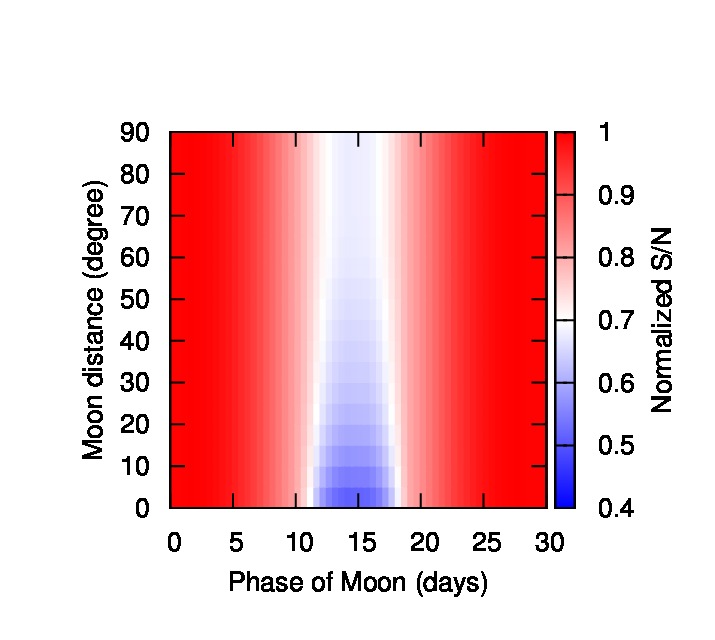
This is a python-based script that is called through a simple cgi web interface. It assumes that the total noise comes from: photon noise, sky brightness level (as a function of Moon phase and distance), and detector properties such as dark current and read-out noise. It also calculates the sky level, on the basis of Moon phase, Moon distance, and selected filters.

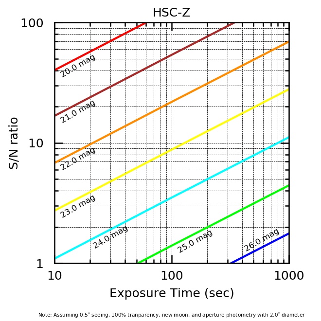
First in “Brightness”, select an appropriate filter and magnitude (in the AB system) of a target. If it is an extended source, use surface brightness in arcsec\(^2\). For a point source, provide a desired seeing value (in arcsec), and for an extended source, a solid angle (size, in arcsec\(^2\)). Next, define observing conditions, namely Transparency (0–1), Moon (days to/from the new Moon, and Moon distance), and (for point sources) the diameter of the aperture that will be used for photometry. Finally, set the maximum sky brightness level (counts, in ADU) to be used in determining the required number of frames.

To calculate an exposure time required to reach a certain S/N, provide a desired S/N and click “Calculate exposure time”. The number of frames is ignored in this option. ETC will compute the total exposure time, limiting magnitude, saturation magnitude (assuming significant non-linearity at 45000 ADU), and the suggested number of frames. If the number of frames is more than 1, the exposure time, limiting magnitude and per frame are also shown. The output also contains the sky level (in ADU/frame). Finally, the total time necessary to complete observations (including overheads) is computed.

To calculate an S/N obtained in a certain exposure time, specify the exposure time in seconds. There are two options; in total or in one frame (the number of frames must be set in the latter). Clicking the “Calculate S/N ratio”button shows an S/N the total exposure time (“Exp Time”\(\times\)number of frames, if such option is chosen) will achieve, as well as in each frame. Total and per frame limiting magnitudes, the saturation magnitude and sky level in ADU, will also be computed. If the number of frames is specified, and the sky level exceeds the maximum value given earlier, we suggest shortening the “Exp Time” and increase the number of frames. If “in total” option is chosen, ETC splits an exposure into multiple frames. Again, the total time necessary to complete observations (with overheads) is also computed.

Currently, ETC does not include dithering patterns. Set the number of frames according to your desired dither pattern. To simulate several exposures per dither position (coadds), the number of frames should be appropriately multiplied. For example: if the pre-defined 5-point dither pattern is desired (i.e., 5 frames) and the resulting sky level is higher than the maximum sky count, set frames to 10, 15, 20, etc.

In addition to ETC, there is also "HSC overhead and required time calculator", which can be used to calculate the total requested time for an observing plan:

https://www.naoj.org/cgi-bin/ohc.cgi

This calculator adds 40 sec per exposure as overheads (detector readout and telescope movement for dithering) and 1.2 hours per night to the total requested time. This latter, operation-related, overhead is shared by all programs, with the amount proportional to the effective on-source exposure time per night. Note that the length of a night is assumed to be 10 hours; therefore, the effective time available for queue observations is (10-1.2) = 8.8 hours. Here, the 1.2 hours per night for the operation-related overheads (calibrations, focusing, filter exchanges and telescope movement) is an average value calculated based on previous observing records. For more information, please refer to

https://www.naoj.org/Instruments/HSC/hsc_queue_overhead.html

Calibrations

QM users will not be charged time (i.e., do not have to include it in Phase 1 or 2) for standard calibrations, which are:

Bias
10 frames per run.
Dark frame
5 frames of 300 sec per run.
Dome flat
in each run, dome flats for all 5 or 6 filters will be obtained

NB: Standard stars

Since the latest HSC pipeline uses the Pan-STARRS catalogue which covers entire skies observable from Hawaii, standard star calibrations are not necessary (some observers may recall that it used to be customary to take one or two short, i.e., 30-sec, exposures in SDSS fields for flux calibration purposes). If you do, however, require some specific standard stars to be observed, please prepare separate OBs. Please note that these additional OBs will be charged (i.e., the allocated time will accordingly be consumed). For OBs requiring narrow- and intermediate-band filters, a nearest spectrophotometric standard star to science fields will be observed immediately before or after science targets and it is free of charge.

Queue proposal template and submission via ProMS

Submission of Subaru proposals is done on-line through the ProMS 2.0 system:

https://proms.naoj.hawaii.edu/proms2/login.php

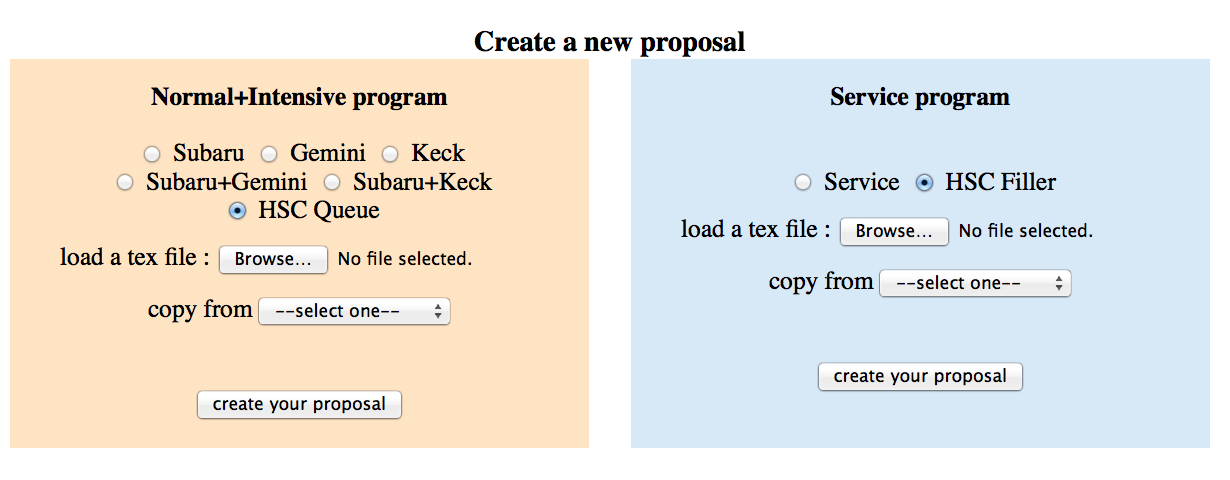
This is a web form that has an embedded template, which is used to create a final pdf document that is sent to the TAC and referees. From this page one can also obtain current semester templates, which can be used to prepare proposals off-line. After login to the ProMS system, one can choose to create a new proposal from scratch, or to load a tex file. One can log in using either the STARS or ProMS ID/password.

**ProMS menu since S17A: *Left*: The “Noral+Intensive program” part, from which the normal HSC QM proposal can be selected. *Right*: QM Filler template, with major differences marked.**

Normal Program

A separate tex template for Normal Queue Mode will be available. Inside the ProMS system, the normal QM proposals can be selected from the field “Normal+Intensive program” (Left figure above). The major difference with respect to the classical mode is box 12. “Observing Run” (Right figure above). Here the PI should give the number of hours (not nights) and specify the observing constraints (see Observing constraints section). The instrument is fixed to “HSC” and no 2nd choice can be given. The total and minimum requested time is also given in hours, not nights. There is no need to have a backup program or provide scheduling requirements other than those necessary to define time constraints.

If time-critical observations are requested, one should write "Time critical" in Comments in Box 12, and provide sufficient information on the time constraint (i.e., acceptable time windows) in Box 13 of the Application Form. If different constraints apply to different targets/fields, one should define the constraints in the list of targets, by adding comments in the "Magnitude" field. Multiple time windows are allowable. The time constraints of the windows should be clearly described, preferably in UT time. The time windows are limited by the number of queue nights in the semester.

Other fields and boxes should be filled similarly to a classical mode program:

https://www.naoj.org/Proposals/howto.html

Intensive Program

The same applies for Intensive proposals as for Normal programs, but the PI needs to uncomment \intensive in box 7 of the application form.

Filler

A separate LaTeX template for Filler Queue Mode will be available. Inside the ProMS system, the filler QM proposals can be selected from the field “Service program” (Left figure above). The template itself is however quite different (Right figure above), and no scientific justification is required for HSC QM fillers. Boxes 1 (Title), 2 (Investigators), 5 (Targets) and 6 (Archive) are the same as for other kinds of applications. The Abstract in box 3 should briefly describe the scientific aim and methods. In box 4 “Observing Run” one should select “HSC’ as the instrument, specify the number of requested hours (\(\le 35\)), and set the transparency, seeing, and filters. Time-critical programs may be acceptable as Fillers, but the chance of OB execution might be small unless the PI sets very relaxed time constraints. Since ProMS cannot accept proposals with identical title, the PIs submitting filler proposals which have similar scientific objectives to their Normal or Intensive proposals have to use a different title.

Evaluation and ranking

Time allocation committee (TAC)

HSC QM proposals will be reviewed by external referees, who will evaluate their scientific content, and by Subaru support astronomers (SAs), who will check the technical feasibility. The time allocation committee (TAC) will then select and rank the proposals based mainly on the referee score. Filler proposals will not be sent to referees, and only the TAC will review them and decide about their acceptance.

Grade

Based on the scientific evaluation, the TAC will assign a Grade to each of the submitted proposals.

Grade A
will be given to QM proposals having a high score. They receive the highest priority to be executed and completed. Even if imcomplete at the end of a semester, they will not be carried over to the next semester. Please reapply if missing data are crucial to the completion of your project.
Grade B
will be given to the rest of accepted HSC QM proposals.
Grade C
will be given to rejected proposals, which, however, will get the permission from the TAC to be observed. In this way the TAC will ensure that there are more programs than necessary to fill the time reserved for QM, which gives more flexibility and backup options during observations. Grade C observations will be performed in good or reasonable weather, when there are no A or B targets.
Grade F
will be given to the Filler proposals, i.e. those intended for bad weather (transparency \(\le 0.4\) and/or seeing \(\ge 1.6''\)). Filler programs might also be executed during classical nights, if there are no adequate backups.

When the constraints of a Grade A, B, or C proposal are found to be too strict, they become a subject of “relaxation”, in order to increase the probability of their execution. This may be requested by the TAC, or by SAs, or even during an observing run (see Changes in OBs).

Acceptance letters (AL)

After the proposal evaluation, each PI will receive an acceptance letter (AL), not later than two weeks after the TAC meeting. AL will include such information as: acceptance judgment, referee score, Grade, and comments from referees and SAs. For Grade B and C proposals, the TAC may request that the observing constraints be relaxed. For Grade F proposals (fillers), the TAC will notify whether the program has been accepted for observations.

Note that proposal Grades may later be published, however referee scores and all comments will only be known to PIs.