Observing blocks (Phase 2)
What are OBs?
Observing blocks (OBs) are the smallest units (quanta) of observations in the queue mode. They describe a single observation, defining the observed object or field, exposure time, dithering pattern (if applicable), and telescope and instrument configuration (filter, position angle, etc.). They also define the constraints, which are used for scheduling the observations – if the current conditions do not meet the criteria given in an OB, such an OB is not executed. There are no limits of the number of OBs for a proposal.
One OB, which includes overheads, should not exceed 30 minutes (1800 sec) of on-source time. In case of Subaru observations one queue OB is translated into one command that is sent to the telescope control system. There is no lower limit for OB total time, and we strongly encourage to make them short, in order to minimize the probability of interrupting one by an emergency situation (sudden weather breakdown, telescope malfunction, etc.). If such situation occurs, the affected OB or exposures will be repeated. However, the general policy is to finish an OB once it has been started.
Due to the specific filter changing procedure, exposures in two filters should be defined as two separate OBs. Two consecutive observations of different exposure times are also not allowed as one OB.
Phase 2 spreadsheet
OBs are prepared using Google spreadsheet. An example and an empty template can be found at Google Docs:
A link to Google spreadsheet for a given proposal, containing the proposal ID and information from Phase 1, will be sent to each PI. It can be edited in a web browser. Observers who have restricted access to Google may contact us and request a Microsoft Excel spreadsheet which can be read and edited in Apache OpenOffice, LibreOffice or similar programs, but should be saved in the .xlsx or .xls format.
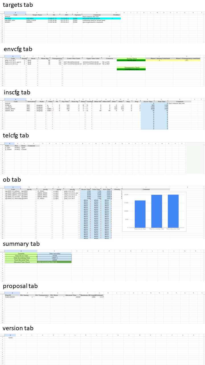
The spreadsheet consists of eight (8) tabs: targets, envcfg, inscfg,
telcfg, ob, summary, proposal and version. They are,
respectively: definition of targets, observing constraints, instrument
and telescope configurations, the OBs themselves, accounting summary
(i.e., time allocated vs. expected time consumed), the constrains
given in Phase 1, and the version info.
The names of tabs and columns must not be changed.
Note that Comment columns should not be used to
describe additional requests and constraints, but only for clarifyiing
notes.
The targets tab
The first tab defines the targets to be observed. Only the targets from
the proposal are allowed, except for special cases of targets approved
by the SOD (see Changes in OBs). In the first column –
Code – one should place an identifier that will later serve
as a reference to this particular target. In the targets
tab as well as the subsequent tabs, only alphanumeric characters
[0-9a-zA-Z] and the underscore symbol “_” and period symbol “.” are
allowed in the Code field. This applies to all Code fields.
For checking and validation purposes, QWG will fill the Target Name
and the RA, DEC fields with the target names
and coordinates, which will be write-protected, based on the information
in the proposal. If there is need to shift the pointing centers, one
needs to define these as new targets below the pre-filled lines. In this
case, one needs to place a new object in the Code and
Target Name fields, and new pointing center coordinates in
the RA, DEC fields. The format hh:mm:ss.ss and
(-)dd:mm:ss.s must be used, respectively. Please note that
Google spreadsheets do not accept strings starting with the hyphen
character “-”. Such strings as, e.g., negative declination, should be
preceded with a single apostrophe (“ ’ ”). The entries in Target Name,
here and in subsequent tabs, may contain blank spaces (e.g.
"My first target"). The Target Name will be the name saved
later in the OBJECT keyword of the FITS file header. The
Equinox should be set in the next column.
If observations of one or more custom standard star fields are desired,
they should be defined as a new targets (new lines), and used
accordingly on the ob tab.
Spectrophotometric standard stars
will be observed for those requesting to use NBFs, and is
free of charge. However, if
specific calibration targets (other than those
listed) are to be desired, this can be
done as described above, but the time will be charged.
The envcfg tab
The second tab defines the restrictions that will be used to decide if the OB can be executed under given observing conditions. Refer to Observing constraints for their explanation.
The cells regarding the seeing and transparency can be edited, but only
to relax the values approved in Phase 1. The Phase 1 values will be
indicated
in the AL, and are also given on the proposal tab. Those cells
cannot be edited.
The column Code is an identifier which can later be used to
refer to a particular set of conditions. One should set the maximum
allowed Seeing, in arcsec. Next, define the sky brightness
in Moon, using dark/gray (HSC runs are not
allocated during bright time). Then, give the minimum allowed separation
from the Moon (Moon Sep, in degrees, 30 for “dark” and not
smaller than 30 for “gray”), and the sky transparency
(Transparency, from 0=“cloudy”, to 1=“completely clear”).
If any of the values in Seeing or Transparency
are stricter than the Phase 1 criteria, an error message will appear.
Seeing must be 0.8, 1.0, 1.3, 1.6, or 100 (i.e., no constraints)
in arcseconds. We also
recommend the following seeing values for each GRADE: equal to or larger
than 1.0 for GRADE A; equal to or larger than 1.3 for GRADE B; and equal
to or larger than 1.6 for GRADE C and F. Similarly,
Transparency must be 0.7, 0.4,
0.1, or 0 (i.e., no constraints). The tolerance factor we use for these
constraints is such that the numbers will be rounded off to the first
decimal place (for example, seeing/transparency 0.84/0.65 for an OB
requesting 0.8/0.7 will be considered good). Note that we define
transparency as the total throughput including the telescope and
instrument, and not just through the atmosphere.
PIs of the Filler proposals must use values equal to or larger than 1.6
in Seeing and equal to or lower than 0.4 in
Transparency.
There are two optional columns, Lower Time Limit and
Upper Time Limit to
define the lower and upper time limits of a time window in the case of
the time critical program. The PI can leave these blank if there are no
time constraints other than the standard visibility defined by the
coordinates. The format follows the standard ISO 8601 regulation, e.g.,
YYYY-MM-DDThh:mm:ss. The default timezone is UTC. For example, the
following forms are permissible: YYYY-MM-DDTHH:MM:SS,
YYYY-MM-DDTHH:MM, YYYY-MM-DD HH:MM:SS, or YYYY-MM-DD HH:MM.
Different timezones can be specified by providing an offset from UTC,
e.g., YYYY-MM-DD HH:MM-10 for Hawaii–Aleutian Time Zone (HAST).
Finally, one can place any additional comments in the last column
(Comment). More than just one set of constraints can be
defined, but none of them can be more restrictive (better seeing, and
transparency, etc.) than the ones requested in the proposal.
The inscfg tab
This tab defines the instrumental parameters used for an OB,
such as filter, exposure time, or dithering pattern. The
Code column defines an identifier which can later be used
to refer to a particular set of parameters. Instrument and
Mode should be kept at “HSC” and “imaging”, respectively.
One should set the Filter, choosing from g/r2/i2/z/Y, or by
typing the name of an NBF. Please use the new filter names
(i.e., r2 and i2, and not r and i).
PA is the
position angle of the
instrument.
Exp Time is the exposure time for one frame, without overheads. The
number of allowed short exposures is limited, so that no more than 5
exposures of 60 sec or less are allowed within a single OB. This limit
does not apply to longer exposures.
Dithering (see Dithering) is defined by
Num Exp, Dither, Dith1, Dith2, Skip and Stop. Note that
there may only be one exposure on a single dither position. To set the
5-point pattern, use Num Exp=5, Dither=5, and
desired values (in arcsec) of the steps \(dRA\) and \(dDEC\) in the
Dith1 and Dith2 columns, respectively. To set
a circular pattern, use Dither=N, and the desired number
of steps in Num Exp. We recommend that this number is kept
around 5. Type the radius of the circle in arcsec in the
Dith1 column, and an initial angle \(\theta\) in degrees in the
Dith2 column. For a single shot (i.e., non-dithering)
exposure, set Dither=1.
In such a case the Num Exp column will define how many
exposures will be obtained without moving the telescope (default is 1).
If one needs more than 5 points in the dither sequence, higher Num Exp
can be set for the circular dither. However, we suggest that
the total amount of time for an OB is kept relatively short,
and it cannot be longer than 30
min (1800 sec) of on-source time. One may choose to split the
configuration in two or more, taking some exposures within the
first one, and the rest within the other. For this, Skip and Stop
should be set appropriately (see
Dithering). Note that
Stop may not be smaller than or equal to Skip.
These separate (but related) configurations must have different Code
identifiers, but must have the same number of Num Exp,
which is the total desired number of exposures in the sequence, as well
as the same values for all other dithering and instrumental parameters.
If a single setting is used, Stop should not be changed –
by default it is equal to Num Exp.
Based on the dithering settings and Exp Time, for each
configuration the spreadsheet will calculate the on-source (without
overheads) and total time (which includes readout time), and
automatically displays them in the On-src Time and
Total Time columns, respectively. These columns should not be
edited.
Guiding=Y for auto-guiding using a guide star, and N for open
tracking. If one wishes to use an offset from the original position
(for example to avoid having the target in a gap between CCDs), these
can be set in Offset RA and Offset DEC
columns, in units of arcsec.
The telcfg tab
This tab defines two configurations, where the dome is open
(Code = “p_opt2”) or closed (“p_closed”). There is no
need to alter anything on this tab.
The ob tab
This tab defines complete OBs, by gathering all the information defined on previous tabs. One line is one OB. Only on this tab PIs may introduce new lines (but not columns) for comments. In this case, the line should be placed in column A and should start with a hash (#).
Code is the name of an OB. It will be used by the
scheduler and telescope control system, so it must be
unique. The drop-down menu bars are used to fill the
next 6 columns, by choosing the codes of the targets, instrument,
telescope (“p_opt2” only) and environmental configurations defined on
previous tabs. The same target can be observed in various
configurations, and a separate line (=OB) is required for each
combination.
If one decides to split the dithering into two configurations, one
should prepare separate OBs for each of them. The On-src Time,
Total Time and Acct (accounting) Time (all in seconds) are
automatically calculated and displayed for a chosen inscfg.
These columns should not
be edited.
Finally, OBs can be prioritized by giving them appropriate numbers in
the column Priority. The lower the number (the lowest is
1), the more important the OB is, and will most likely be executed
earlier. Several or even all OBs may have the same
Priority. Prioritizing may be useful in case of programs
in which more targets were defined in Phase 1 than are expected to be
observed. If standard star observations are defined, it is important
to give them at least the same or slightly better priorities than
those given to intended science fields so that they would be executed
at the same time or as close in time to each other as possible.
The box on the right illustrates the total
on-source time that has been programmed (total of the
On-src Time column), the total accounting time adds
readout time per frame, and overhead time required for
the queue-mode operation, and compares it with the total time allocated
by the TAC (automatically loaded from the proposal tab).
From S21A, the allocated time includes all overhead time.
The summary tab
This tab summarises what is shown graphically on the ob tab
regarding various time (total on-source, accounting, and allocated
time).
If the total
accounting time exceeds the allocated time, a warning message will
appear in red, but such a situation is allowed. These
fields should not be modified.
The proposal tab
This tab shows the ID of the program, the amount
of allocated time, and the strictest observational constraints, as
defined in Phase 1 (i.e., proposal). While different values can be used for
these constraints in the envcfg tab, the new values cannot
be stricter than the values defined here (i.e., in the original proposal).
This tab is predefined, so it must not be modified.
The version tab
This tab only contains the version ID (e.g., S24A). There is nothing to be done here but please make sure that the latest version is always used.
Finding charts
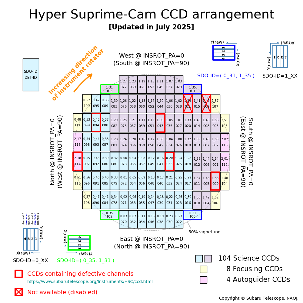
There is no dedicated tool for finding charts (FC) preparation at the time of writing. Nevertheless, in Phase 2, PIs are responsible for providing correct target coordinates. In order to check the coordinates of the fields, and whether or not the targets fall in the gaps between the chips, or onto a failed CCD channel, there are a couple of choices available:
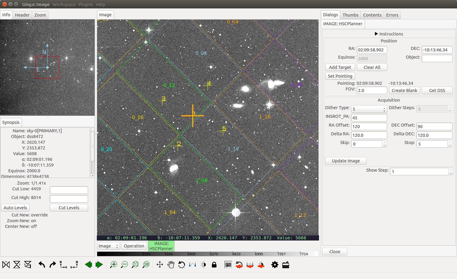
First option is to use the Ginga fits viewer, with an additional HSCPlanner plugin:
https://hscq.naoj.hawaii.edu/HSCPlanner/
The plugin helps to visualize a field with a dither on the HSC CCD plane (see an example view of HSCPlanner plugin below). The detailed instruction of installation and use, including a tutorial video, are available at the link above.
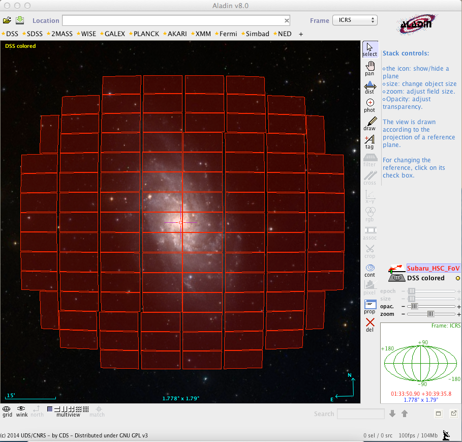
One can also use an Aladin FoV file:
https://www.naoj.org/Observing/queue/img/Subaru_HSC_FoV.xml,
and plot it over a sky image from a selected image server (see an example view of Aladin display below). Detailed instructions can be found here:
https://www.naoj.org/Observing/queue/misc/hsc_field_check_aladin/
OB check and submission
The deadline for OB submission (end of Phase 2) is the same as that for Service proposals. OB submission is done through the following website:
https://hscq.naoj.hawaii.edu/qcheck
This tool should first be used to check if an OB is correct and ready to be submitted (despite some validity test solutions already implemented in the spreadsheets). PIs are responsible for the validity and correctness of their OBs.
To use the check tool, type the name of your spreadsheet in the box provided, then click “Check”. The system will list all the errors and warnings found, as shown in the example linked below:
https://www.naoj.org/Observing/queue/ph2-check-warning-explained.pdf
An OB cannot be submitted if errors are present. Warnings do not prevent from OB submission, but the PI should make sure the information in the spreadsheet are correct.
Apart from using this tool, one should check that the codes within each
tab are unique, especially those in the first column of the
ob tab. Check, in particular, that there are no targets
that were not listed in the proposal, and that the observing constraints
are stricter than those specified in the original proposal. Also, make sure
that no OB exceeds 30 min of on-source time. However it is allowed to
prepare OBs that use more total time than allocated by the TAC. This is
to allow for some flexibility and backup options during the
observations. Note that the time spent on the program will never
exceed be the allocated time, and therefore in this case some OBs will
not be
executed. For Intensive Programs, PIs can submit OBs planned for the
following semesters, which can be executed when there is a chance for
early execution.
To use the submission tool, log in using your STARS username and
password (ProMS ID will not work). If this is your first
Subaru proposal, the STARS account will be set up, and information will
be sent in a separate email. In case of doubts or questions, contact
![]() .
.
If correctly logged-in, a “STARS Login succeeded” message will appear. One session lasts for 3 hours, and there is no need to log in again during that time. Input your spreadsheet’s name in the box at the top and click “Submit’. After submission, each spreadsheet will be double-checked for errors and consistency with the proposal, i.e., if they do not exceed the allocated time, if the constraints are the same, etc. If inconsistencies are found, they must be corrected.
It is possible to list all the spreadsheets and OBs that have already been submitted. Simply type the ID of your proposal in the “Proposal ID” field, and click “List files”.
We encourage PIs to submit their observations as early as possible.
This will give the observatory more time for consistency check,
communicating necessary corrections, simulatiing schedule, and will also
allow for possible early execution (see
Early execution).
We will not
accept Phase 2 submission after the deadline without an agreement
between PI and QWG. If you are willing to proceed to Phase 2, but will
not be able to submit the Phase 2 sheet by the deadline, please contact
![]() .
.
Grade C and F Phase 2 submissions will be reviewed but their results will not be communicated to their PIs. Submitted versions of Phase 2 will be more or less accepted as they are. If any obvious errors are found, they will be corrected without any correspondence with PIs.
Changes in OBs
Please carefully prepare OBs, as opportunities for making changes after their submission are limited. Until Phase 2 is finalised, PIs can consult with us to modify exposure times, or loosen observing constraints. We may also proactively contact PIs in Phase 2 and ask for some modifications to be made.
Except for relaxing constraints, major changes are not possible once Phase 2 is finalised and OBs are sent to the scheduler. To relax constraints after Phase 2 is finalised (in order to increase the probability of execution), PIs should contact SOD first. If permission is granted, re-submission is possible for those OBs that had not been executed yet.
Other changes are not allowed, except in special cases. If an original target needs to be changed, SOD must be consulted first. It may be allowed if the science goal is unchanged, there is no conflict with other programs (see also Clearly prohibited cases), and there is a good reason. Changing filters must also be discussed with SOD first.