Observing transits
Transit predictions from the Exoplanet Transit Database.
High precision Photometry for Exoplanet transit
Olivier Guyon, Frantz Martinache
Detection of transiting exoplanets requires high precision photometry, at the percent level for giant planets and at the ~1e-5 level for detection of Earth-like rocky planets. Space provides an ideally stable - but costly - environment for high precision photometry. Achieving high precision photometry on a large number of sources from the ground is thus scientifically valuable, but also very challenging, due to multiple sources of errors. We show that these errors can be greatly reduced if a large number of small wide field telescopes is used with a data reduction algorithm free of systematic errors. The recent availability of low cost high performance digital single lens reflex (DSLR) cameras provides an interesting opportunity for exoplanet transit detection. We have recently assembled a prototype DSLR-based robotic imaging system for astronomy, showing that robotic high imaging quality units can be build at a small cost (under $10000 per square deg square meter of Etendue), allowing multiple units to be built and operated. We demonstrate that a newly developed data reduction algorithm can overcome detector sampling and color issues, and allow precision photometry with these systems, approaching the limit set by photon noise and scintillation noise - which can both average as the inverse square root of etendue. We conclude that for identification of a large number of exoplanets, a ground-based distributed system consisting of multiple DSLR-based units is a scientifically valuable cost-effective approach.
1. Introduction: Challenges to high precision photometry of a large number of sources
The table below lists the challenges to achieving high precision photometry of a large number of sources. The sources of errors fall in three broad categories:
- Photon noise is a fundamental limit, common to both space and ground. For a transit survey, it can only be mitigated by the survey etendue (product of collecting area and field of view), regardless of how this etendue is achieved (many individual units pointing in the same direction or a single unit).
- Atmospheric effects can reduce both the efficiency of the survey (fraction of cloudy weather) and its accuracy (differential extinction, color effects, PSF variations coupled with instrument). A fundamental limitation is imposed by scintillation, which cannot easily be calibrated (it is largely incoherent between sources in a wide field image), and can therefore be most efficiently mitigated by survey etendue. At fixed etendue, atmospheric effects are best reduced if multiple units are used, as most atmospheric effects are decorrelated between units (scintillation, PSF shape). Variation in sky extinctions will favor geographically separated units.
- Instrumental effects need to be compensated for by proper calibration and data reduction. They can be mitigated by deploying multiple units, provided that instrumental errors are uncorrelated between units.
| Error term | Solution, mitigation strategy |
| Atmospheric Scintillation | Large etendue, multiple units, multicolor imaging |
|---|
| Weather, daytime | Multiple sites, good sites |
|---|
| Photon noise | Large etendue, small PSF (for faint sources only) |
|---|
| Variable extinction | Multiple sites, calibration, multicolor imaging |
|---|
| Static detector defects | Stable pointing, calibration, multiple units |
|---|
| Dynamic detector defects | Calibration, multiple units |
|---|
| Tracking errors | Guiding, Calibration, multiple units |
|---|
| Differential tip-tilt | multiple units, large instrumental PSF |
|---|
| PSF variations | large instrumental PSF, multiple units |
|---|
| Source blending, confusion | calibration, PSF shape analysis, multicolor imaging, small PSF |
|---|
Almost all of the instrumental errors are highly unlikely to be correlated between separate units (with the exception of variable extinction, weather, daytime interruptions and source blending/confusion). The strategy we chose to adopt for a successful transit survey consisting is therefore to:
- (1) Achieve a large etendue per unit, and deploy multiple units, if possible at multiple sites. The final photometric accuracy is achieved by averaging by averaging the measurements from several units to achieve the final required precision. This is a cost per etendue challenge, and we discuss in section 2.
- (2) Reduce, for each unit, the instrumental error - if possible down to the limit imposed by non-instrumental error sources (scintillation, photon noise, variable extinction). This is calibration challenge, and we discuss our approach to solve it in section 3.
To validate this approach, a prototype was assembled and operated since Jan 2011 at the Mauna Loa observatory located in Hawaii, USA. The prototype, described in section 2, relies on inexpensive commercially available hardware.
2. Demonstrating low cost, high reliability and large etendue with a commercial DSLR camera based system
2.1. Main choices and prototype system description
A description of the system can be found on this page .
2.2. Detector characterization: are low cost commercial CMOS detectors suitable ?
A description of the measured detector performance can be found on this page .
2.3. Keeping the cost down
2.3.1. Implementation cost
The combination of a DSLR camera with a high quality commercial lens offers a very attractive cost per etendue compared to more conventional hardware used in astronomy (CCD camera + custom optics). The total system cost must also include other hardware such as mount, electronics and computer, which must be taken into consideration during design to keep the cost low. A detailed cost assessment for the prototype 1 is provided on this page. The total cost for the system, including manpower, is estimated at $14000, with $7713 in hardware and $5600 in manpower (assuming $100 per hr).
Prototype 2, which is currently starting operation, is somewhat cheaper per etendue, thanks to the fact that two cameras are now mounted on the same mount and share the same computer. The total cost for prototype 2 is about $18000 including manpower, which comes out to $9000 per camera.
Fabrication of multiple unit may slightly reduce the cost per unit by reducing manpower requirement per unit and sharing hardware (for example, 4 cameras could be mounted on the same mount). A lower limit of approximately $5000 per camera seems reasonable if many units are fabricated, given that each camera + lens costs almost $3000, and that there are practical limits to how much other hardware can be shared and how little manpower can be devoted to each unit (assembly of components, software installation, troubleshooting scale with number of units). Since each camera offers 0.6 deg2m2 of etendue, the cost per etendue is close to $9000 / deg2m2.
2.3.2. Operation cost
Keeping the operation cost low requires fully robotic operation of the units and low failure rate, requiring very infrequent maintenance (or no maintenance at all). Failure is defined here as any event which requires physical intervention (computer reboot at site, replacement of a part). With multiple units, some level of failure rate can be tolerated with little increase in operation cost. For example, a failure rate of 10% of the units per year may be acceptable, as a visit to the site every 2 yrs would maintain most of the units functional. Our ongoing work with the prototype system is essential to converge to a system design with high reliability: reliability needs to first be demonstrated on a single (or a small number of) unit(s), and failure points in the design then need to be identified and addressed prior to building and deploying multiple units.
A concern for the operation cost is the large volume of data that needs to be transfered and processed (approximately 2.5GB per night per camera). For a single unit, this data volume is manageable with the network bandwidth available at most observatories, but deployment of a large number of units requires careful planing of data management.
2.4. Lessons learned with prototype 1
2.4.1. System reliability
From late December 2010 to July 2011, our first single camera prototype was in operation at Mauna Loa observatory. The prototype was successfully operated fully robotically from March 2011 to July 2011. In July 2011, the prototype was removed from the site to start upgrade to prototype 2.
During the full period (Jan to July 2011), there was one failure requiring visit to the site, when a lightning storm stopped power to the system for longer than the ~6 hr capacity of the system's UPS. The system's computer needed to be physically accessed for reboot (no automatic reboot). There was also an incident requiring remote login to the system: during a snow storm, some water found its way in a connector carrying a DC voltage meant to inform the system about the AC power health ahead of the UPS. This lowered the DC voltage below the threshold, and placed the system into safe mode (camera pointing down, to avoid complete stop when the camera is pointing up). This second problem was temporary solved by lowering the voltage threshold in the software, and was later permanently solved by improving the seal around the connector.
2.4.2. System performance
The system performance was satisfactory except for pointing, due in part to the equatorial mount electronics and to the fact that our prototype 1 was mounted on the side wall of a wooden building. While the mount worked reliably, the electronics driving the stepper motors and the communication protocol to the electronics did not easily allow high performance tracking. This problem, combined with the fact that the mounting on a wooden wall did not provide a very stable reference, let to large drifts in pointing (approximately 1" to 5" per mn).
This issue is addressed in our second prototype by:
- Mounting the unit on a sturdy metal frame, directly bolted to a ground concrete pad
- Replacing the native mount electronics with stepper controller+driver circuits offering more fine control of pointing and tracking (allowing for example small updates in tracking speed without introducing unwanted jumps/interruptions in the tracking)
- Implementing closed loop guiding: the images acquired are continuously used to refine pointing and tracking
3. Calibrating instrumental errors with the Remove, Replace and Compare (RRC) algorithm
3.1. Description photometric data reduction approach and challenges
Our photometric measurement is differential: other stars in the field are used to construct a reference against which the target star is compared. Choosing the optimal of PSF(s) used for comparison with the target star is essential to compensate for error terms correlated with other sources (variable extinction due to clouds and airmass, color effects, detector non-linearity). The choice of the comparison PSFs is therefore critical to achieving photometric precision, and is complicated by the detector's undersampling of the PSF, discussed in the next paragraph.
The main challenge to precision photometry with a low-cost DSLR-based system is to overcome errors due to PSF sampling, which are particularly serious in our system, as the pixel size is comparable to the PSF size, and the pixels are colored (25% of pixels are red-sensitive, 50% are green-sensitive and 25% are blue-sensitive). This issue could be mitigated by defocusing the image, thus spreading light of each star on many pixels. For example, defocusing star images to a 35 pixel diameter disk, Littlefield (2010) report achieving 1% photometric accuracy in each of the 3 detector color channels over 90 sec exposures with a 203 mm telescope, and measuring transit depth to 0.1% (1 millimagnitude) for a 1hr duration transit. While this scheme is appropriate for photometry of a small number of bright stars, it is not suitable for a transit survey aimed at monitoring a large number of stars, as the combined loss of angular resolution (crowding limit) and faint-end sensitivity (mixing starlight with background) would have a large impact on the survey performance.
In addition to the PSF sampling issue, a large number of variables can affect the measured apparent flux from stars (for example airmass, color extinction effects, PSF variations). Comparison PSF(s) used for differential photometry must be chosen to include these effects, either by choosing stars which are subjected to the same errors, or by understanding, modeling and compensating for these effects.
3.2. Modeling vs. Statistical "Lucky PSF" approach
The challenges listed in the previous section could be addressed by PSF modeling and analysis of sources of photometric error, as is often done for precision photometry with imaging arrays. This analysis would constrain both the choice of the ideal comparison PSF(s) to perform differential photometry, and how to compensate for residual errors. For example, the effect of PSF color on the photometric signal could be estimated (either empirically from the data or by modeling), the colors of PSFs in the field estimated, and the best comparison PSFs could be then be chosen according to this analysis. Other effects would be treated in a similar way, and the final choice of the comparison PSF would rely on combining the results of several such analyses. The PSF undersampling issue would be mitigated by PSF shape modeling and analysis of how PSF location at the sub-pixel scale affects the photometric measurement.
A simpler and more powerful approach is to use the large number of PSFs in the field to automatically select the best comparison PSFs with no modeling of errors. The target PSF images acquired before and after (but not during) the transit to be tested are compared with all other PSF images in the field, and the selection of the best comparison PSF(s) is based upon choosing PSF(s) that best matches the target PSF images. The selection is not affected by the transit, as the image(s) of the target during the transit are not used for the selection. This technique uses the powerful statistical argument that in a sequence of wide field images, there must be at least one "Lucky" PSF which experiences the same errors as the target (a PSF which has the same brightness, same color, falls on the same fractional pixel position, etc...). Rather that trying to identify such PSF(s) by measuring relevant parameters (color, PSF position, etc..) and relying on model(s) to understand how these parameters affect the photometric measurement, our algorithm empirically perform the identification by comparing images, and does not require know ledge of what are the physical processes producing errors in the photometry. As detailed in section 3.3, this selection must be done at the image level, and should not be done at the lightcurve level: since multiple sources of errors contribute to an aperture photometry measurement, several independent effects might cancel each other in the aperture photometry data (for example PSF shape, color, pointing) during the set of images used for identification of the reference PSF(s), while they would not cancel during the transit.
3.3. Why use PSF images comparison instead of lightcurves ?
A large number of effects can induce instrumental photometric measurement errors in an imaging system, including PSF shape (through its interaction with pixels), color, tracking errors, location on the image (through atmospheric extinction), local environment (are there nearby PSF(s) in the images, which may partially overlap with the target image), local pixel properties (such as pixel-to-pixel variations in sensitivity and color response). The amplitude of these effects, their time and spatial properties, and interdependancies are generally poorly known. Mathematically, the measured target flux Fmeasured, obtained through summation of pixel intensities can thus be written as:
|
Fmeasured = f(Freal, p1, p2, p3, p4 ... pn )
|
(1)
|
|---|
where p1, p2, p3 ... pn are parameters affecting the measurement (tracking error, airmass, PSFshape, inter-pixel sensitivity variations, intra-pixel sensitivity variations, nearby image structures, etc...). The measurement process is mathematically equivalent to a mapping of a n+1 dimension space onto a 1-D measurement space. Some of the parameters are fixed in time (stellar color for example) while others are time variable (airmass, sub-pixel position of the target in the presence of tracking errors).
LINEARIZE ?
Thankfully, for most of these parameters, the effect is correlated (or anti-correlated) between sources in the field. For example, pointing error in the RA direction may introduce a positive error on the target and an equally negative error on a separate source.
Detrending techniques of photometric light curves .
- The Curse of dimensionality. With several parameters affecting the photometric measurement, the volume corresponding to possible realizations of these parameters rapidly becomes too large to be sampled by calibration stars, even in a deep wide field image.
- Coupling between parameters.
These issues can lead to the choice of bad calibration sources.
Example: Effect of instrument focus correlated with pointing.
3.4. Algorithm description
3.4.1. Testing transits instead of working from lightcurves
The algorithm we propose to use does not rely on building a light curve and then identifying transits in the light curve (as is usually done). Instead, we seek to test a transit hypothesis for a given choice of transit parameters (transit duration and phase): did a transit occur at phase phi, period P, and of durationd d ?.
The metric computed is the estimated transit depth for this particular choice of transit parameters. We scan the transit parameters (phase, period and duration) to measure the estimated transit depth across the 3-D space defined by the parameters. If no transit occurs, the resulting 3-D map contains noise, with approximately as many positive values as negative values.
This approach offers fundamental advantages over the conventional approach of working from lightcurves. The optimal data analysis parameters should ideally be a function of the transit parameters, but a lightcurve based approach fixes these parameters across the time span during which the lightcurve is computed. Detrending techniques are aimed at mitigating this limitation, but do not offer full flexibility. For example, the choice of the best PSFs for comparison should ideally maximize correlation between the target PSF and reference PSF(s) excluding the time during which the transit occurs. As the transit phase or duration changes, the criteria for the choice of the best reference PSF(s) will therefore also change, and the algorithm should ideally be able to pick different comparison PSF(s) as these parameters change.
3.4.2. Step by step description of the algorithm
- STEP 1 - Choose a set of transit parameters (phase, period and duration). The purpose of the steps below is to test if the transit matching these parameters occured. The metric used is the transit depth, computed at the end of the steps.
- STEP 2 - Separate the images of the sequence in two groups: group A consists of all images during the transit, group B consists of all the images outside the transit.
- STEP 3 - Use all images in group B (outside transit) to identify PSF(s) in the field which best match the target PSF. The identification is done directly from the images (no photometry, no lightcurve), using the sum square difference between target images and PSFs as a minimization criteria. For example, the following criteria may be used:
|
V(ii,jj) = SUMi=0..n-1 [ SUM|ii12+jj12 < radius2| (Bi(ii0+ii1,jj0+jj1)-Bi(ii+ii1,jj+jj1))2 ]
|
(1)
|
|---|
where i is the image index within set B, n is the number of images in set B, Bi(ii,jj) is the pixel value for pixel (ii,jj) in image i within the group B, (ii0,jj0) is the location of the target star, and radius denotes the size over which the pixels are compared. The value V(ii,jj) then represents how well, within the group B of images, the pixel values around pixel (ii,jj) match the pixel values around pixel (ii0,jj0) - where the target star is located. We note that V(ii0.jj0)=0, and that a small value for V(ii,jj) indicates that a star which behaves similarly to the target star is located on pixel (ii,jj). Equation (1) may be refined to include flux scaling (allow for comparison of stars of difference brightnesses), and weighting factors that take into account noise properties (readout noise, photon noise) or other known limitations.
- STEP 4 - Construct a reference PSF image sequence during the transit. The value(s) of (ii,jj) for which V(ii,jj) is smallest is(are) used to build this sequence. For example, if the single smallest value of V(ii,jj) (other than the trivial ii=ii0, jj=jj0 solution) is obtained for (ii,jj)=(iimin, jjmin), then :
|
RefPSFj(ii,jj) = α Aj(ii+iimin,jj+jjmin)
|
(2)
|
|---|
where α is adjusted to best match the photometry of the target and reference PSF outside transit (group B), and j is the image index within group B (during transit).
- STEP 5 - Derive the estimated transit depth a by comparison of the target PSF and reference PSF during transit. An estimate of the transit depth a may be obtained by:
|
(1+a) = (SUMj=0..m-1 SUM|ii12+jj12 < radius2| Aj(ii0+ii1,jj0+jj1) ) / (SUMj=0..m-1 SUM|ii12+jj12 < radius2| RefPSFj(ii1,jj1) )
|
(3)
|
|---|
Where m is the number of images in group A. This equation may be improved by optimal weighting of pixel values.
4. Preliminary on-sky result
4.1. Test dataset
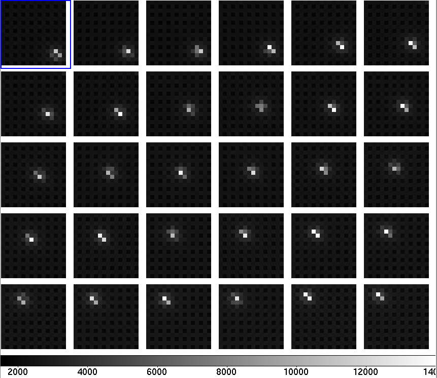
The star HD 54743 (mV = 9.39) was observed on 2011-04-15 (UT) with the robotic imaging system described in section 2. Figure 1 shows a single full frame image, and figures 2 and 3 show the region surrounding HD 54743 with increasing detail. Thirty consecutive 65-sec exposures were acquired at ISO100, as shown in figure 4. The images were acquired during bright time, with a relatively strong background (level = 2500 ADU, 2600 ADU and 1900 ADU per pixel per exposure in R, G and B respectively).
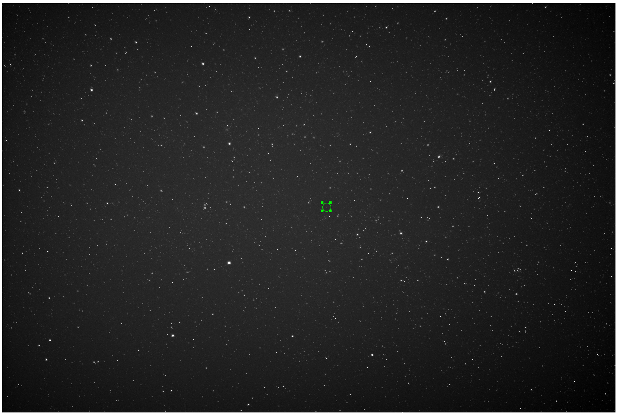 |
HD 54743
Figure 1: Full frame single 65-sec image of the HD 54743 field (10 x 15 deg). The small green circle shows the location of HD 54743.
|
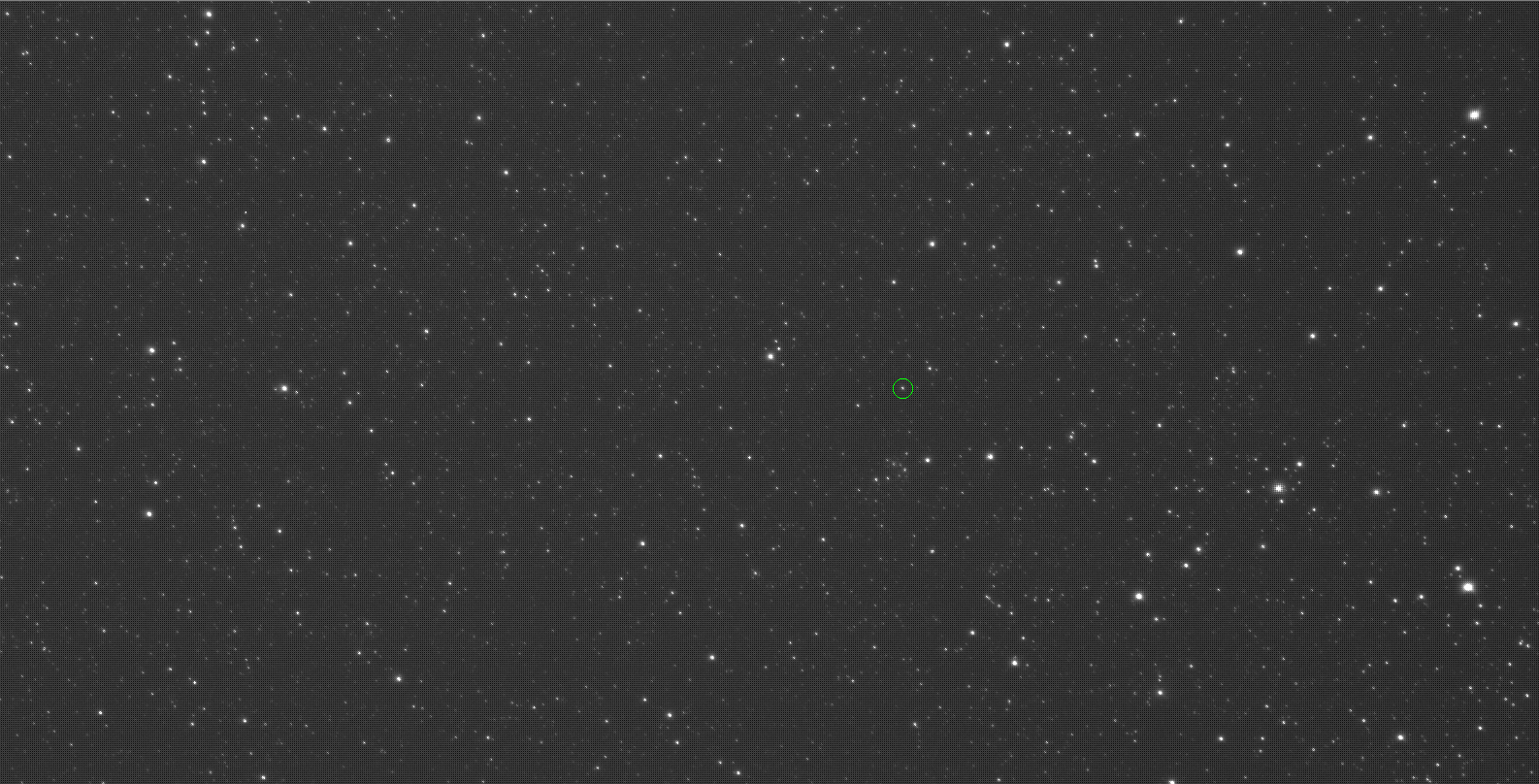 |
Figure 2: Part of the above image, showing the location of HD 54743. The small green circle shows the location of HD 54743.
|
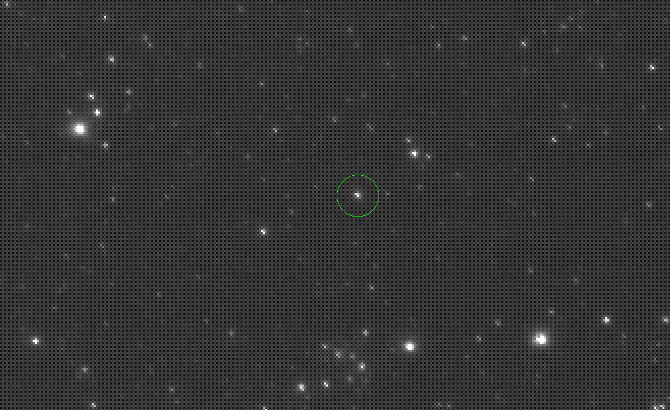 |
Figure 3: Part of the above image, showing the location of HD 54743. Individual pixels are visible. The green circle shows the location of HD 54743.
|
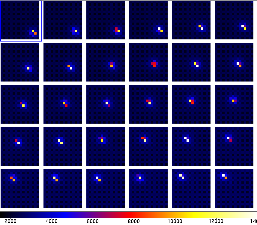 |
Figure 4: Sequence of 30 consecutive RAW images, showing the 16 pixel x 16 pixel detector area around star HD54743. The Bayer color array is visible in the raw data: the dark background pixels (1 pixel out of 4) are the B channel, and the brighest background pixels are the G channel (1 pixel out of two); the remaining pixels are the R channel.
A B&W version of this figure is here.
|
This dataset is especially challenging for photometry, as the PSF is strongly undersampled (in part due to the fact that the camera's anti-aliasing filter has been removed), the detector is a color CMOS array, and the tracking is relatively poor, with a drift of approximately 5" per minute (0.5 pixel between consecutive frames).
4.2. Conventional Aperture photometry
Aperture photometry results for the dataset are shown in Figure 5 and the table below (showing standard deviation). The measured standard deviation in each of the 3 color channels is significantly larger (2x to 6x depending on the color) than the combined effect of known fundamental noises (photon noise, readout noise, scintillation and flat field error). This is due to the undersampling of the PSF by the color detector array. Figure 4 shows that the PSF is about one pixel wide, and that if it is centered on a pixel, the corresponding color will be artificially enhanced in aperture photometry.
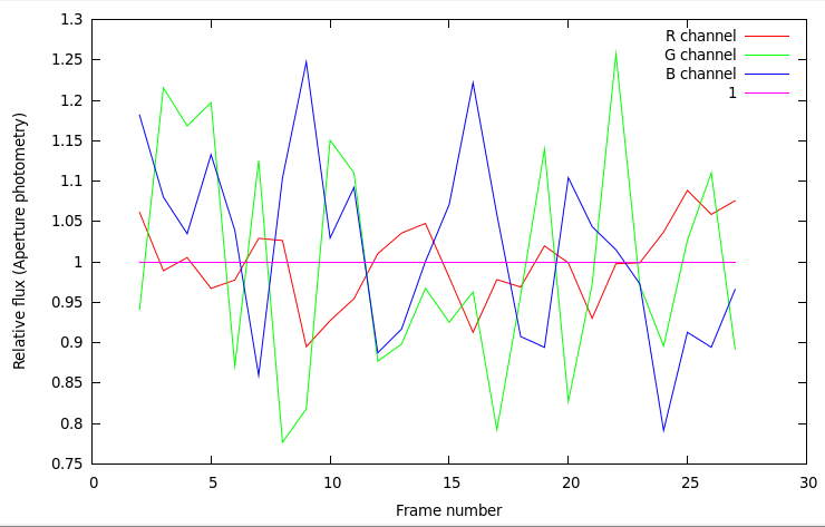 |
Figure 5: Aperture photometry derived from the raw data shown in Figure 4. A 4 pixel radius mask (=40") was used, with the background computed for each of the 3 color channels using pixels outside the aperture mask.
|
| R channel | G channel | B channel |
| Average count (ADU) | 5918.04 | 25990.6 | 6658.04 |
| Standard Deviation | 4.72% | 13.56% | 11.24% |
Since the standard deviation is dominated by this sampling effect, the values in the table above can be interpreted as a measure of this effect alone. Interestingly, the R channel standard deviation is smaller than either the G or B channels. Close inspection of the data shows that this is due to the fact that the PSF is wider in the R band than in other colors, and sampling errors are therefore smaller in this band. The sampling error is largest in the G channel, even though this channel has twice as many pixels as either R or B channels: the PSF is much sharper in the G color than other colors.
4.3. Aperture Photometry with RRC algorithm
The dataset was processed with the RRC algorithm. For each image i in the dataset, the assumption to be tested was: "Did a transit occur during, and only during, frame #i". Group A (during transit) therefore consists of frame #i, and group B (outside transit) consists of all other frames. For each i, the transit depth was estimated.
Figure 6 shows a key step in the algorithm, with i=15. The target PSF during the hypothetical transit is shown on the left: this is the data that is removed. All other data (other frames + frame number 15 excluding the target PSF) is then used to build an estimate of what the target PSF should be on frame 15. This template is shown on the right part of the figure, and replaces the missing data. Comparison of the removed data and replacement leads to a photometric estimate of the transit depth, if the transit occurred during frame number 15. In this particular example, the template is built from a linear combination of 80 other PSFs in the field.
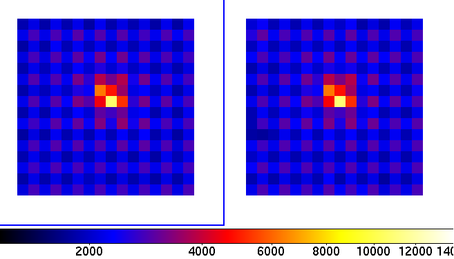 |
Figure 6: Left: Target PSF number 15 (HD 54743 image extracted from frame number 15 - this PSF can also be seen in Figure 4, noting that index starts at 0 at the top left of the figure). Right: Template reconstructed from other PSFs in the field. The template is compared to target PSF number 15 to derive photometry. The template is obtained from a linear combination of PSFs other than the target, and the linear coefficients used to build it were computed after removal of target PSF 15 from the dataset. Derivation of the template shown on the right is therefore fully independent of the target PSF number 15 shown on the left. The match between the two PSFs is good at the few percent level.
|
Figure 7 shows the estimate transit depth for each frame number using the RRC algorithm, and can be directly compared with Figure 5 (aperture photometry).
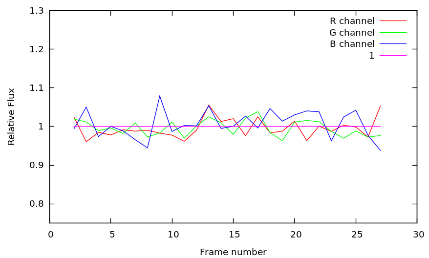 |
Figure 7: Photometry with the RRC algorithm, with a 65 second time averaging (one single exposure). A 4 pixel radius mask (=40") was used for the final photometry step. The scale is the same as Figure 5.
|
| Error term | R channel | G channel | B channel | Notes |
| Atmospheric Scintillation | 0.3% | 0.3% | 0.3% | |
|---|
| Photon Noise | 2.79% | 1.00% | 2.24% | mV=9.35, includes background contribution (bright time, r=40arcsec mask) |
|---|
| Readout Noise | 0.40% | 0.23% | 0.71% |
|---|
| Flat field error | 0.5% | 0.4% | 0.5% | Error term irrelevant with good tracking |
|---|
| Total (expected) | 2.88% | 1.14% | 2.42% |
| Achieved | 2.48% | 2.04% | 3.51% |
The achieved photometric precision in each color channel is given in the table above: it is at the photon noise limit level for the R channel, 60% above photon noise limit for the B channel and at twice the photon noise limit in the G channel. The expected photometric precision, assuming no PSF sampling error term, is given for comparison, and shows that our algorithm reduces sampling errors at the level of, or below, other dominant sources or errors.
5. Discussion
The success of an exoplanet transit survey program relies on the ability to monitor a large number of targets with high photometric precision. While space-based missions have the advantage of providing a highly stable environment, a large number of units can be deployed inexpensively on the ground to average down errors and weather. The keys to achieving high photometric precision in a ground-based transit survey are therefore to (1) deploy a large number of reliable robotic units at a competitive cost and (2) reduce for each unit the noise level, if possible approaching or reaching the photon noise limit. Assuming that noise can be reduced to the fundamental limit imposed by photon noise, the performance of an exoplanet transit survey is then entirely driven by total etendue (product of field of view by collecting area multiplied by the number of units). This edendue can then be allocated to a deep survey of a small fraction of the sky or a shallower survery of a large fraction of the sky, depending on the scientific goals.
We have shown in this paper that commercially available digital single lens reflex (DSLR) cameras using low noise CMOS arrays offer a highly reliable and cost-effective approach to obtain large etendue, at a cost below $10k per square meter square deg of etendue. Our results demonstrate that (1) these low cost cameras can be scientifically valuable thanks to attractive detector performance (low noise), (2) a robotic DSLR-based system can be build and operated reliably at a small cost and with a small failure rate, and (3) a statistical approach to photometry analysis of wide field images can almost eliminate sampling and color effects in DSLR cameras, turning them into high precision photometers. Together, these three points demonstrate the value of an approach where a high number of DSLR-based units, potentially similar to the prototype described in this paper, would perform a photometric survey of a large fraction of the sky.


