Nulling interferometry

A nulling interferometer is defined by its aperture geometry (number, positions and sizes of its subapertures) and the coherent beam combinations performed between subapertures to produce the intereferometer output beams. In this study, the optimal choice of aperture geometry is discussed for the detection and characterization of exoplanets. Solving this problem is made possible by the existence, for any aperture geometry, of a single optimal beam combiner design, as established in a previous study. A signal-to-noise based performance criteria is used to identify optimal geometries in several cases relevant to detection and spectral characterization of exoplanets.

The analysis presented in this paper results in several important findings for the design of nulling interferometers:

Optimal interferometer geometries tend to follow supernuller configurations, in which the subaperture positions follow specific geometrical laws allowing deeper nulls than possible in the general 2-D case: lines, circles or arcs, hyperbolas.
When the geometry is enforced to be circular (all apertures on a circle), the optimal interferometer geometry is one where the spacing between consecutive apertures is constant.

Several new high performance nulling interferometer designs are proposed and discussed:

A 6-aperture 1-D interferometer delivering excellent starlight rejection and robustness to pointing errors and cophasing errors: 3 out of the 6 output beams have stellar leak level below 1e-8 for a stellar radius of 0.1 λ/D (below 1e-10 for two of the output beams). [png]
An 8-aperture 2-D circular geometry interferometer offering 5 out of 8 outputs with starlight rejection better than 1e-8 for a 0.01 λ/B radius star. Three of these outputs are darker than 1e-10, and one of them stays below 1e-10 for stellar angular radius up to ~0.1 λ/D. This interferometer is particularly sensitive for the observation of Earth-like planets in visible light. [png]
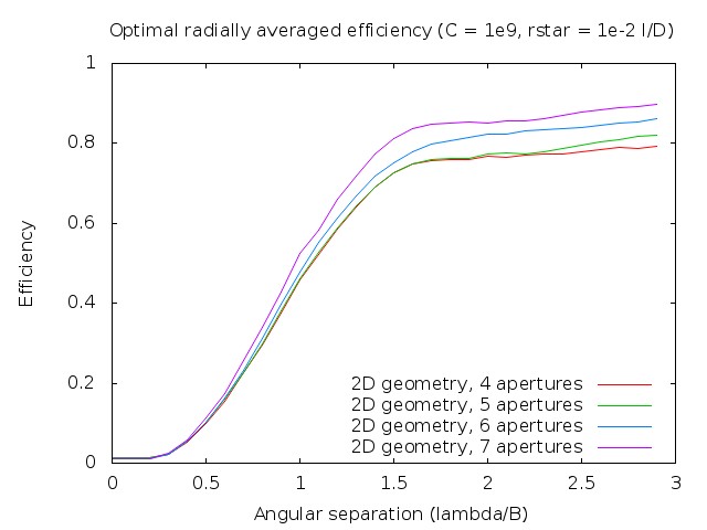
A 7-aperture geometry consisting of a regular hexagon and a central aperture. For 4 out of its 7 outputs, the starlight rejection is better than 1e-8 for a 0.01 λ/B radius star. [png]

1. Introduction

Nulling interferometers consist of an array of telescopes coherently combined in order to produce output beam(s) in which starlight is strongly suppressed. These outputs allow detection and characterization of exoplanets around nearby stars. Nulling interferometers are especially attractive if the angular resolution required to separate the planet(s) from its host star is too challenging to achieve with a single aperture telescope. For example, unambiguous direct detection of Earth-like planets around nearby stars requires ~0.05" angular resolution, requiring a 40m baseline at 10μm wavelength. At shorter wavelength, nulling interferometers can allow cost-efficient approaches to exoplanet imaging and characterization [ref DaVinci].

The performance of a nulling interferometer is a function of both the geometry of its entrance aperture and the design of its beam combiner. While many designs have been suggested to achieve deep extinction of the partially resolved stellar disk, the optimality of such designs has not previously been addressed, and it remains unknown if designs proposed so far can be significantly improved, or if they are nearly optimal. Recent studies have started to answer key questions about the performance limits of nulling interferometers and are providing valuable insights to improving their designs. [Rouan] showed that arbitrarely deep nulls can be produced provided that a sufficient number of telescopes is used. In a recent study, the optimal design of a beam combiner for a nulling interferometer was addressed, proposing a technique to optimally design a beam combiner, and showing the existence of a minimum achievable null depth which is only a function of the number of apertures. These studies are focused on achieving deep nulls, and do not take into account the sensitivity of the interferometer in realistic observing problems. They also do not provide guidance as to the optimal array geometry and how it drives the nulling interferometer performance.

The goal of this study is to establish, for a range relevent observation scenarios and constraints, what is the optimal nulling interferometer design, and to quantify its performance for direct imaging of exoplanets, relative to previously proposed nulling interferometer designs. This work builds on the technique to optimally design a nulling beam combiner, as it allows considerable reduction of the number of degrees of freedom when searching for an optimal nulling interferometer design: the full design of the nulling interferometer is only a function of its aperture geometry. A signal-to-noise (SNR) based metric to evaluate the performance of a given nulling interferometer design is first introduced and discussed in section 2. Section 3 describes the numerical approach taken to identify optimal nulling interferometer designs, identifying four specific observation scenarios and providing a few examples. In Section 4, results from an exhaustive search of optimal nulling interferometers are presented and summarized.

2. Quantifying nulling interferometer performance with the signal-to-noise ratio (SNR) factor

2.1. Requirements

The two most commonly used metrics for the performance of a nulling interferometer are:

Null depth : Ideally, a nulling interferometer should be able, on at least one of its output, to remove most of the starlight. While reaching infinite nulling depth (perfect removal of the central source's light) is conceptually possible for a point source, maintaining a deep null is challenging on a partially resolved stellar disk. The interferometer's ability to maintain deep nulls on partially resolved stellar disks is often quantified by the null order which describes how light leakage varies as a function of angular separation θ to the optical axis for a point source. In a second-order null interferometer, the light at the output of the interferometer is a second-order function of the angular separation to the optical axis (the null is then said to be in θ²).
Interferometer throughput : As much as possible, a large fraction of the planet's flux should be preserved to allow its detection and characterization. Interferometers can be very inefficient, as light from multiple apertures is combined into numerous interferometric outputs, and only one or a few of the outputs may be used toward detection, as the other outputs contain too much starlight. Many nulling interferometers only produce one nulled output, and the amount of planet light in this output is a function of planet offset to the optical axis, leading to a interferometric "transmission map" showing peaks or fringes of high throughput while the position-averaged throughput is low.

The first metric (null depth) quantifies how well the interferometer can reject starlight without consideration for its efficiency (= interferometer throughput). Optimizing for null depth alone yields designs in which successive beam combinations increase resilience to stellar size at the expense of efficiency, as only a single (or very few) interferometer output(s) are part of the final measurement, with the other outputs being discarded: they are necessary intermediate steps toward reaching a deep null but they contain too much starlight. A nulling interferometer should simultaneously offer high rejection of starlight and high throughput.

For a given configuration (star diameter, planet to star contrast, planet position and interferometer design), each output of the interferometer contains both starlight and planet light. In this paper, a signal-to-noise (SNR) based definition of the nulling interferometer's performance is adopted, which includes all outputs of the interferometer and optimally weights them according to their individual SNR. This performance metric optimally balances null depth with throughput, and is physically representative of the interferometer's ability to detect and characterize exoplanets. With the SNR-based performance metric, quantitative comparisons between interferometers can be made, such as comparing the exposure times required for a given exoplanet detection between two designs. The SNR-based performance metric is described quantitatively in section 2.2.

2.2. Measuring the interferometer's performance with the SNR factor

In this section, the measurement of the interferometer's performance is described. It is first assumed that an interferometer design is adopted, consisting of its aperture geometry and its nulling device represented as a unitary matrix U (as described in a previous study) which transforms the complex amplitude at the interferometer's entrance into the complex amplitude at the output of the beam combiner. It is assumed that the interferometer is pointed at a star+planet system. The star is C times brighter than the planet with the contrast C >> 1. The angular radius of the star is rs (<< 1 radian). The interferometer's intensity response to the star and planet are each N-element vectors :

I(star)_m = set of N intensity outputs for the star alone (m=0..N-1)
I(planet)_m = set of N intensity outputs for the planet alone (m=0..N-1)

To take into account the stellar angular size, the star is modeled as a series of mutually incoherent points, each represented by a complex amplitude vector V(α,β) where α, β are the point coordinates on the sky relative to the optical axis, and the coefficients of V are the complex amplitude values at each of the array's subapertures. The intensity vectors I=|UV|² at the output of the interferometer are computed separately for each point and then summed to compute the interferometer's intensity response I(star) to the partially resolved stellar disk.

The total flux is preserved through the interferometer:

Istar = ∑_m=0..N-1I(star)_m = total starlight gathered by the interferometer (2.1)

Iplanet = ∑_m=0..N-1I(planet)_m = total planet light gathered by the interferometer (2.2)

To measure the interferometer's performance, the planet detection SNR is evaluated on each of the N interferometer outputs:

SNR_m = I(planet)_m / sqrt( I(planet)_m + I(star)_m )	(2.3)

The overall SNR is then obtained by the quadratic sum of the SNRs on the individual ouputs :

SNR = sqrt ( ∑_m=0...N-1 SNR_m² )	(2.4)

The SNR obtained in equation (2.4) is compared to the SNR that would be obtained if the central star did not exist. If there is no star (Istar = 0), equations (2.3) and (2.4) lead to :

SNR0_m = sqrt(I(planet)_m)	(2.5)

which, using flux conservation, leads to:

SNR0 = sqrt(Iplanet)	(2.6)

The interferometer's SNR factor is defined as the ratio of SNRs from equations (2.4) and (2.6):

SNRfactor = SNR/SNR0	(2.7)

The SNR factor is thus a unitless number which quantifies how the planet detection SNR is affected by the stellar flux:

SNRfactor=1 means that the interferometer has successfully isolated starlight from planet light, and the planet detection sensitivity is not affected by starlight
SNRfactor=0.5 means that the addition of starlight divides the planet detection SNR by 2. The exposure time required to reach a given sensitivity is multiplied by 4 compared to the SNRfactor=1 case.
SNRfactor close to zero means that the interferometer has not been able to separate planet light and starlight, and the planet is much harder (impossible ?) to detect than it would be without the star

At high contrast (C>>1), equation (2.3) shows that the key to achieving high SNRfactor is to have the planet flux and the starlight in different outputs of the interferometer. SNRfactor quantifies how well the interferometer can separate the two fluxes. SNRfactor is a function of the interferometer geometry, the interferometric combinations made (matrix U), the contrast C, the stellar angular size, and the position of the planet relative to the star. It is not a function of integration time or total collecting area; it is therefore a quantitative measurement of how optimal the interferometer design is.

2.3. Uniform incoherent background (zodiacal light)

While zodiacal light is not considered in this study, its effect on the optimal design of a nulling interferometer is qualitatively described in this section.

2.3.1. How is background light processed by the nulling interferometer ?

A background light component with no spatial structure is fully incoherent, and will not interfere between separate apertures of the interferometer. For example, with equal area subapertures each of the N outputs of the interferometer will exhibit a background level equal to the total background flux collected by each subaperture over the subaperture PSF area on the sky. In the more general case of unequal area subapertures, the background flux will still be spread over all outputs, as incoherence between apertures makes it impossible to concentrate background flux on a small fraction of the interferometer's outputs.

2.3.2. How much incoherent light is mixed with the planet light ?: comparison with a single aperture telescope

In an interferometer of maximum baseline B, the contribution of the incoherent background due to zodiacal light is larger than for a full aperture telescope of diameter B, and can be larger than the planet light contribution.

In a full aperture telescope of diameter D, the amount of zodiacal light mixed with the planet signal is obtained by multiplying the zodiacal background level by the telescope collecting area and the PSF area and it therefore equal to :
I_zodi = B π (D/2)²/(λ/D)² = B A_telescope / (λ/D)² , (2.8)
where A_telescope is the collecting area of the telescope. The amount of planet light collected is:
I_planet = A_telescope F_planet , (2.9)
where F_planet is the incident flux from the planet.
In an interferometer consisting of N apertures, each of diameter d, with a full interferometer diameter D, the amount of zodiacal light per output is B π(d/2)²/(λ/d)², and the total amount of zodiacal light mixed with the planet light is therefore :
I_zodi = B γ N π (d/2)² / (λ/d)² = B γ A_{interferometer} / (λ/d)² = B γ A_{interferometer} (D/d)² / (λ/D)², (2.10)
where A_{interferometer} = N π (d/2)² is the total collecting area of the interferometer and γ ranges from 1/N (all planet light is in a single output of the interferometer) to 1.0 (planet light is equally distributed between all outputs of the interferometer). The amount of planet light collected is:
I_planet = A_{interferometer} F_planet , (2.11)
where F_planet is the incident flux from the planet.

Interferometer vs. single aperture telescope of same collecting area : With the same collecting area (= same total flux collected from the planet) for both the single aperture and the interferometer (d=D/sqrt(N)), and assuming the most favorable case for the interferometer (γ=1/N), the interferometer and single aperture telescope mix the same amount of zodiacal light with the planet light. In a less favorable configuration (γ>1/N), more zodiacal light is mixed with planet light in the interferometer.
Interferometer vs. single aperture telescope of same diameter : For the single aperture telescope:

I_planet/I_zodi = F_planet (λ/D)² /(B),	(2.12)

while for the interferometer,

I_planet/I_zodi = F_planet (λ/D)² /(B γ (D/d)²).	(2.13)

Comparison between equations (2.12) and (2.13) shows that in the interferometer, there is considerably more mixing of zodiacal light with planet light, as γ (D/d)² > 1, even for γ=1/N.

2.3.3. Impact on optimal interferometer design

With a zodiacal background component, equation (2.3) becomes:

SNR_m = I(planet)_m / sqrt( I(planet)_m + I(star)_m + I(zodi)),	(2.14)

where I(zodi) is the amount of zodiacal background collected by each subaperture over the solid angle of a subaperture's PSF. As described in section 2.3.1., I(zodi) is the same for all interferometer outputs and is independent of d (the d² dependence of the collecting area and the d^-2 dependence of the subaperture PSF solid angle cancel). On the other hand, I(planet)_m is proportional to d². The presence of zodiacal light will therefore push the interferometer design toward:

Larger collecting area. Since I(zodi) is independent of d, but both I(planet)_m and I(star)_m are proportional to d², the relative contribution of the zodiacal background can be reduced by increasing the diameter d of each subaperture.
Better concentration of the planet light in a few interferometric outputs. I(zodi) is independent of the interferometer beam combination design and is uniformly distributed among all outputs of the interferometer, unlike both I(star)_m and I(planet)_m. The impact of the zodiacal background can be reduced by concentrating as much planet light as possible in a few outputs. This would need to be achieved for most possible positions of the planet on the sky. A good example of an optical system which achieves good concentration of the planet flux in a few outputs is a single aperture imaging telescope, where the planet's flux is concentrated in a few pixels.

3. Approach to optimizing nulling interferometer designs

3.1. Observational scenarios considered

Four examples, representative of scientifically valuable high contrast imaging problems, are used to evaluate the interferometer performance in this study:

Case 1: Search of Earth-like planets with a IR interferometer . The star to planet contrast is 1e6, the stellar radius = 1e-2 λ/D, and the performance metric used is the quadratically average SNR factor for all planet position within a 2 λ/D radius
Case 2: Imaging & spectroscopy of small separation (0.7 λ/D) planets (Jupiter, Earths) with an IR interferometer. The contrast is 1e6 and the stellar angular radius is 1e-3 λ/D. The performance metric is the quadratically averaged SNR factor on a 0.7 λ/D radius circle.
Case 3: Search of Earth-like planets with a visible interferometer. The contrast is 1e9, the stellar radius is 1e-2 λ/D, and the angular separation is less than 2 λ/D. The performance metric used is the quadratically averaged SNR factor for all planet position within a 2 λ/D radius
Case 4: Search of planets with a visible interferometer at small angular separation. The contrast is 1e9, and the stellar radius is 1e-3 λ/D. The performance metric is the quadratically averaged SNR factor on a 0.7 λ/D radius circle.

TABLE 1: Observation scenarios
	Description	Contrast	Stellar radius	Scoring region
1	Search of Earth-like planets with a IR interferometer	1e6	0.01 λ/B	r < 2 λ/B
2	Imaging & spectroscopy of small separation planets (Jupiter, Earths) with an IR interferometer	1e6	0.001 λ/B	r = 0.7 λ/B
3	Search of Earth-like planets with a visible interferometer	1e9	0.01 λ/B	r < 2 λ/B
4	Search of planets with a visible interferometer at small angular separation	1e9	0.001 λ/B	r = 0.7 λ/B

In each case, the metric used to measure the nulling interferometer performance is the quadratically averaged SNR factor over the scoring region:
SNR = sqrt( 1/n Σ_i=1ⁱ⁼ⁿ SNR_i²) (3.1)
This value represents the effective SNR in the hypothetical scenario where many observations are combined, with the planet at a different location within the scoring region for each observation and a constant probability density function for the planet location within the scoring region. This hypothesis is representative of actual observations, due to the combined effect of planet orbital motion, changes in the interferometer position angle, and, for a polychromatic observation, chromatic evolution of the λ/B separation metric used. The inverse square of the quadratically averaged SNR factor is proportional to the total exposure time required to detect the planet (or characterize it to a given level). For example, if the quadratically averaged SNR factor is 0.5, the detection will require 4 times as much exposure time as the "no star present" case.

3.2. Numerical code

Figure 3.1 shows the main algorithm steps to evaluate the performance of an nulling interferometer geometry. First, the optimal beam combiner is designed following the technique descriped in this study . A transmission map I_k(α,β) of the interferometer is then constructed for each ouput k of the beam combiner. With knowledge of the stellar angular size, the stellar intensity output is computed for each output by integration of the transmission map I_k(α,β) over the stellar disk α²+β² < rs². For each output of the interferometer, a map of the SNR is then computed at fixed star-to-planet contrast value. The SNR maps (one map per interferometer output) are then combined into a single SNR map, which can then be quadratically averaged within the scoring region to produce the performance metric.

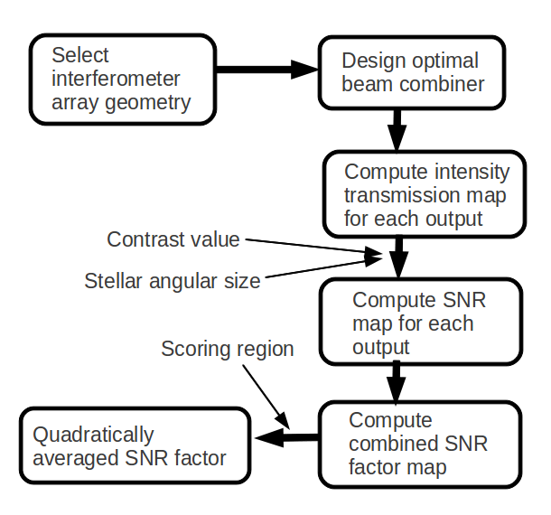Figure 3.1: Main algorithm steps from definition of the interferometer geometry to computation of the quadratically averaged SNR.

A simulated annealing algorithm is used to search for optimal array geometries. The current best array geometry is perturbed, the new performance value computed and compared to the previous best value, and a probabilistic decision is then taken to move to the new point or stay at the current point depending on the difference between the two values, following the simulated annealing minimization scheme.

3.3. Example: Optimal 4-aperture nulling interferometer design

3.3.1. Previously proposed 4-aperture nulling interferometer design

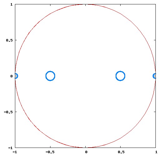Figure 3.2: Four subaperture 1-D nulling interferometer design geometry from Angel & Woolf 1997.

A four aperture 1-D design was proposed by Angel & Woolf (1997) to offer a 6th order null (it is denoted AW97 from now on). In this double Bracewell configuration, the dark outputs of two Bracewell interferometers are combined to produce the deep null. The central pair baseline is half of the outer pair baseline, and the central pair uses apertures twice the radius of the outer pair apertures. The interferometer geometry is :

Aperture 0 : (-0.999998 -0) 0.316228
Aperture 1 : (-0.499999 -0) 0.632456
Aperture 2 : (0.499999 0) 0.632456
Aperture 3 : (0.999998 0) 0.316228

For each aperture, the numbers in parentheses are the (x y) coordinates, and the last number is the aperture radius.

The quadratically averaged SNR factors for this array are computed with the algorithm described in section 3.2., yielding the following values:

Case 1: 0.592548
Case 2: 0.529287
Case 3: 0.59353
Case 3: 0.341332

3.3.2. Optimal 4-aperture designs

The numerical code is used to look for the optimal 1-D four apertures (free aperture diameters) nulling interferometer with the same observation parameters. Results are written in files such as Aper4_SSize20_C9.txt.

Case 1: IR search for Earth-like planets
The optimal 1D geometry (free aperture diameters) gives:

cp ./RESULTS_1DDIFFDIAM/Aper4_SSize20_C6_AVERAGE.txt f1.txt
./plotgeom f1.txt 0

Stellar size = 0.01
Contrast = 1e+06
SNR factor = 0.748716
Separation = 0
Aperture 0 : (-1 0) 0.420499
Aperture 1 : (1 0) 0.420169
Aperture 2 : (-0.311719 0) 0.568697
Aperture 3 : (0.312794 0) 0.568526

This new geometry, shown in the Figure below, is 1.6 times more efficient (requires 1/1.6 times the exposure time) than the AW97 geometry.

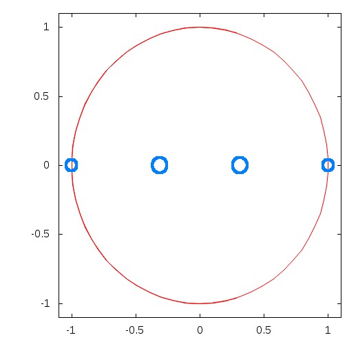Figure 3.3: Optimal 4 aperture nulling interferometer geometry for the observation of a faint companion (10⁶ contrast) located within 2 λ/B from a central source of radius 10^-2 λ/B. This geometry was chosen to maximize the quadratically averaged SNR factor. The optimization led to a design similar to AW97, but with slightly smaller central apertures on a smaller baseline.

The optimal 2D geometry (free aperture diameters) gives:

./plotgeom ./RESULTS_DIFFDIAM/Aper4_SSize20_C6_AVERAGE.txt 0

4 Apertures
Stellar size = 0.01
Contrast = 1e+06
SNR factor = 0.746532
Separation = 0
Aperture 0 : (0.502948 0.864317) 0.420157
Aperture 1 : (-0.512971 -0.858406) 0.42132
Aperture 2 : (0.159603 0.268765) 0.568124
Aperture 3 : (-0.172561 -0.260849) 0.5685

This geometry is also a 1-D geometry, and is identical (within numerical precision of the code) to the optimal 1D geometry obtained above. This is a direct consequence of the fundamental superiority of linear arrays to reach deep nulls with a small number of apertures: a nulling interferometer with 4 apertures can only produce a 4th order null if it is linear.

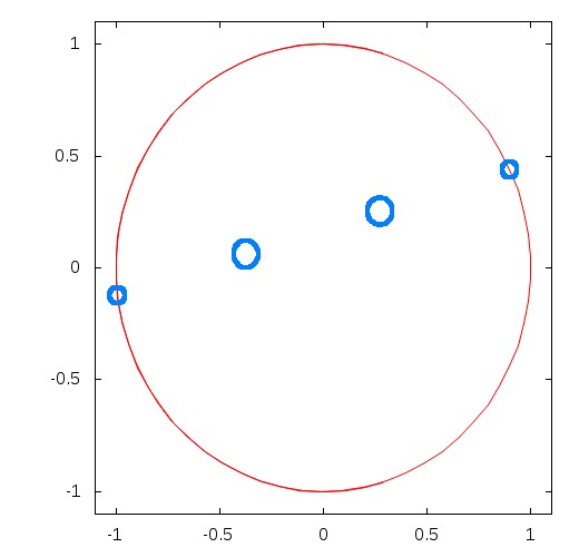
Case 2: Small IWA imaging & spectroscopy of planets (Jupiter, Earths) with IR interferometer
The optimal 2D geometry (free aperture diameters) gives:

./plotgeom ./RESULTS_DIFFDIAM/Aper4_SSize30_C6_ave.txt 7

4 Apertures
Stellar size = 0.001
Contrast = 1e+06
SNR factor = 0.746883
Separation = 0.7
Aperture 0 : (0.381207 -0.924485) 0.49996
Aperture 1 : (-0.38408 0.9233) 0.500056
Aperture 2 : (0.917292 0.398205) 0.499829
Aperture 3 : (-0.92473 -0.380625) 0.500154

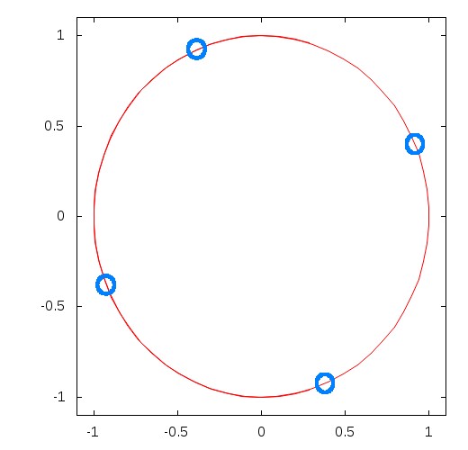Optimal 4 apertures interferometer geometry for the observation of 1e6 contrast source at 0.7 λ/D.

In this case, the small stellar size (1e-3 λ/D in radius) does not require a 4th order null at 1e6 contrast: the optimal geometry is not linear, and apertures are pushed to the edge of the circle to offer maximum efficiency at sub λ/D separation. This geometry offers twice the efficiency of the AW97 geometry for this observation.
With a 1D geometry, the optimal geometry SNR factor would be 0.607, and would produce a 3-apertures interferometer:

./plotgeom ./RESULTS_1DDIFFDIAM/Aper4_SSize30_C6_ave.txt 7

4 Apertures
Stellar size = 0.001
Contrast = 1e+06
SNR factor = 0.607168
Separation = 0.7
Aperture 0 : (1 0) 0.53349
Aperture 1 : (-1 0) 0.533129
Aperture 2 : (0.000323114 0) 0.532541
Aperture 3 : (0.001844 0) 0.384137

Optimal 4 apertures linear interferometer geometry for the observation of 1e6 contrast source at 0.7 λ/D.

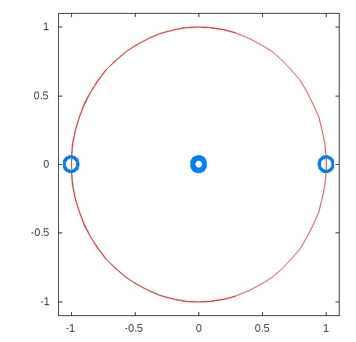
Case 3: Search of Earth-like planets with a visible interferometer

./plotgeom ./RESULTS_DIFFDIAM/Aper4_SSize20_C9_AVERAGE.txt 0

4 Apertures
Stellar size = 0.01
Contrast = 1e+09
SNR factor = 0.612783
Separation = 0
Aperture 0 : (-0.99222 -0.124493) 0.370785
Aperture 1 : (0.274229 0.251621) 0.603242
Aperture 2 : (0.89932 0.437291) 0.365548
Aperture 3 : (-0.371366 0.0598244) 0.604146

Optimal 4 apertures interferometer geometry for the observation of 1e9 contrast source within 2 λ/D.

Case 4: Small IWA search of planets with a visible interferometer.

./plotgeom ./RESULTS_DIFFDIAM/Aper4_SSize30_C9_ave.txt 7

4 Apertures
Stellar size = 0.001
Contrast = 1e+09
SNR factor = 0.577962
Separation = 0.7
Aperture 0 : (-0.0804094 0.996762) 0.518494
Aperture 1 : (-0.999789 0.0205558) 0.508443
Aperture 2 : (0.0887336 -0.996055) 0.482549
Aperture 3 : (0.988885 0.148681) 0.489691

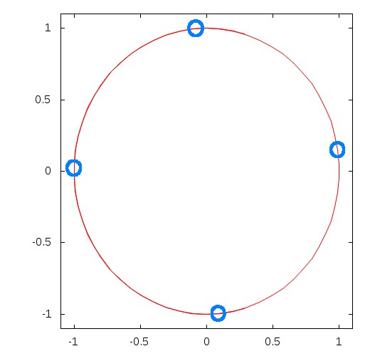Optimal 4 apertures interferometer geometry for the observation of 1e9 contrast source at 0.7 λ/D.

3.3.3. Discussion

The linear AW97 4-aperture array design is close to being optimal

4. Results of an exhaustive search of optimal nulling interferometer designs

4.1. Number of apertures and geometry constraints

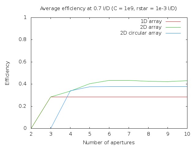
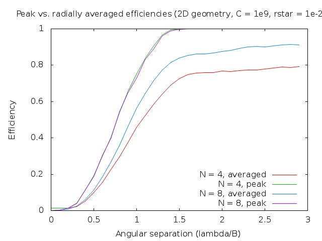
The next 4 figures show for each of the 4 cases considered, what is the impact of number of apertures on the nulling interferometer's efficiency. The efficiency is defined as the square of the SNR factor, and is therefore inverse proportional to the exposure time required to reach a fixed signal-to-noise.

Efficiency as a function of number of apertures for case 1 (1e6 contrast, stellar radius = 1e-2 λ/D, averaged efficiency within a 2 λ/D distance from the star)

Efficiency as a function of number of apertures for case 2 (1e6 contrast, stellar radius = 1e-3 λ/D, averaged efficiency at 0.7 λ/D distance from the star)

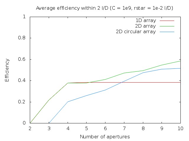Efficiency as a function of number of apertures for case 3 (1e9 contrast, stellar radius = 1e-2 λ/D, averaged efficiency within a 2 λ/D distance from the star)

Efficiency as a function of number of apertures for case 4 (1e9 contrast, stellar radius = 1e-3 λ/D, averaged efficiency at 0.7 λ/D distance from the star)

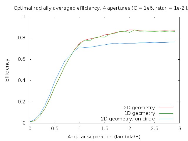
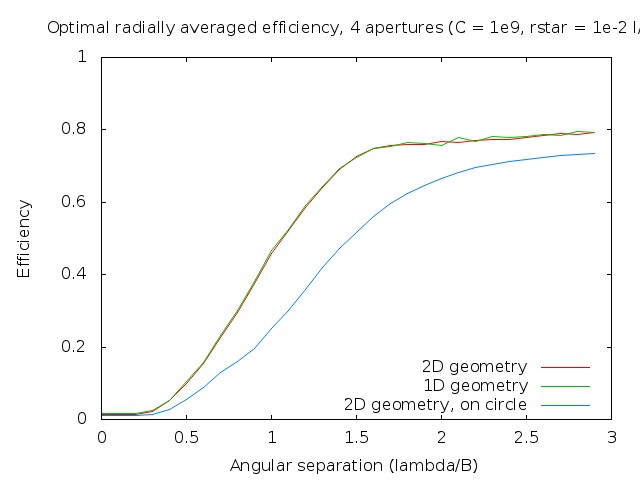
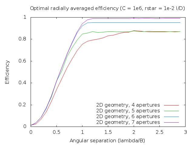
4.2. Efficiency as a function of angular separation

Peak vs. radially averaged efficiency

Conclusion

The analysis performed in this paper relies on a simple model for the target, consisting of a partially resolved stellar disk and an unresolved planet. Using the planet detection signal-to-noise ratio in the photon noise regime as a metric, it is then possible to find the optimal interferometer geometry and beam combination scheme given geometry constraints such as maximum baseline, array shape (linear, circular, or general 2D) and number of apertures. The impact of exozodiacal light was not considered, but may also drive the optimal array geometry [Defrere et al 2010].

References, links

Olivier Absil's paper on nulling interferometer configurations

Page content last updated: 27/06/2023 06:35:52 HST
html file generated 27/06/2023 06:34:39 HST