Nulling interferometry

Home

Optimal beam combiner design for nulling interferometers

Summary

• (1) There exists a well defined minimum achievable null depth for a 2-D nulling interferometer, which is only a function of number of apertures. Although deeper nulls may be achievable in special cases (such as for a linear array), the location and sizes of the apertures has not effect on the interferometer's null depth in the general 2-D case, although it affects the amount of planet light that can be directed to the nulled output(s).
• (2) Deeper nulls can be achieved with 1-D interferometer geometries than possible with 2-D geometries with the same number of apertures. Any 1-D interferometer with N apertures can achieve a 2(N-1)-order null, while the order of the deepest null for a random geometry 2-D geometry interferometer is the order of the N-th term in the Taylor expansion of e^i(x2+y2) around x=0, y=0 (2nd order null for N=2,3; 4th order null for N=4,5,6, etc...).
• (3) An optimal beam combiner for nulling interferometry relies only 0 and π phase shifts

1. Introduction

Spectral characterization of Earth-like planets around other stars may reveal the presence of life, and is therefore of high scientific value. Acquiring a high quality spectra of small rocky planet in the habitable zone around its host star requires an instrument that can optically separate starlight from planet light in order to avoid being limited by photon noise from the host star. Two approaches have been studied in the last few decades: nulling interferometry with an array of telescopes, and single aperture coronagraphy. A nulling interferometer is an interferometer designed to cancel light from an on-axis source (usually a star) while keeping as much as possible light from faint sources close to the central star. Nulling interferometers can thus detect light from exoplanets [Bracewell 1978] , and are particularly attractive at infrared wavelengths (about 10 μm) for which the planet to star contrast is more favorable than in visible light. At this wavelength, a single aperture (+coronagraph) option would require a large telescope due to the linear dependence of angular resolution with wavelength, and an interferometer consisting of widely separated telescopes is a more suitable approach [Bracewell 1979][Woolf & Angel 1986]. Nulling interferometers with short (few meter) baselines have also been proposed for visible light observations of exoplanets [Shao & Levine 2010].

A key limitation of the two-telescope nulling interferometer proposed by [Bracewell 1978] is due to the finite angular size of stars, which, even in the absence of instrumental defects, makes it impossible to fully cancel starlight while preserving light from a faint nearby source (planet). With a 2-telescope configuration, the ideal nulling interferometer throughput for a point source is proportional to the square of the angular separation to the optical axis: the interferometer produces a second order null near the optical axis, commonly referred to as a θ² null, where θ is the angular separation to the optical axis. Since stellar diameters are typically about 1 percent of the planet to star separation for a system similar to the Earth-Sun system, the maximum differential attenuation between starlight and planet light attainable with a 2-telescope design is therefore around 1e4, short of the ~1e6 (thermal IR) to ~1e10 (visible light) contrast between the two objects.

To overcome this limitation, nulling interferometers with more than two telescopes have been proposed to achieve higher order nulls, thus offering better extinction on partially resolved stellar disks. The extinction is then a function of both the interferometer geometry and the interferometric combination between the telescope beams [Lawson et al. 1999], and many interferometer designs have been proposed, with increasing null depth. The Angel Cross design [Angel 1990] combines for example two Bracewell interferometers in a 2-D geometry to achieve a θ⁴ null. Angel & Woolf 1997 later showed that a linear 4-aperture design can offer a θ⁶ null. With 5 telescopes, a solution offering a θ⁸ deep null was also proposed [Woolf & Angel 1997]. [Leger et al. 1996] and [Mennesson & Mariotti 1997] established array geometry requirements to reach a given nulling order, and proposed a 5-telescopes solution offering a deep null and able to distinguish the signal from a planet from a symetrical exozodiacal cloud. Rouan 2003 shows that arbitrarily deep nulls can be obtained, given a sufficient number of telescopes, and discusses in a later paper [Rouan 2006] the practical usefulness of deep nulls, finding that interferometers with deeper null are more resilient to phase errors.

Null depth is unfortunately often achieved at the expense of efficiency: for a fixed number of apertures, a smaller fraction of the total light gathered by the interferometer is used as null depth is increased. For example, in the 4-aperture Angel Cross design, 25% of the light is used (only one of the four interferometer outputs offers the θ⁴ null depth), while a simpler 2-aperture Bracewell offers 50% throughput with a θ² null. Null depth and throughput must therefore be balanced to find the optimal interferometer design when total mission cost/complexity are taken into account, and the scientific return of the mission must be maximized. Consequently, the optimal array geometry may not offer a very deep null in order to maintain high throughput, or to adopt an aperture geometry which can be easily realized, such as maintaining all apertures on a circle to avoid long delay lines. For example, the Darwin mission study adopted a 4-aperture geometry on a circle, with a 2nd order null [Cockell et al. 2009], with a 50% efficiency (two of the four interferometer outputs are used for science), and for which stellar leakage is about 100 times brighter than light from an Earth-like planet at 10pc.

It is therefore important to understand how the achievable null depth and throughput are constrained by aperture geometry, to simultaneously optimize the aperture geometry and beam combiner design. This interferometer optimization problem however remains largely unsolved, as the development of new nulling interferometers designs has been so far iterative, with no single design method leading to improvements, and no clear understanding of where the performance limits might be, given array geometry constraints. The relative importance of array geometry and beam combiner design is especially unclear, as previously published nulling interferometers designs rely on a particular match between aperture positions and beam combinations to achieve deep nulls, making it impossible to decouple their relative impact on performance. The goal of this paper is to provide a universal method to optimally design the beam combiner for any nulling interferometer geometry, and thus to establish performance limits of nulling interferometry given realistic array constraints (such as maximum number of telescope, or maximum baseline). To achieve this goal, a universal mathematical model of the interferometer is first established and described in section 2. This model is then used in section 3 to derive, for a given entrance aperture geometry, the optimal beam combiner design. Nulling interferometer design examples are given in section 4 to illustrate the findings of this paper.

2. Nulling interferometer model

2.1. Relationship with Coronagraphy

Traditionally, coronagraphs use single aperture pupil (which may be composed of adjacent segments) and perform starlight rejection with masks introducing amplitude and/or phase in pupil and/or focal planes. Nulling interferometers use a sparse array of telescopes, and perform starlight rejection by coherent destructive interference between the beams. The boundaries between the two techniques have become less clear as several authors have suggested using nulling interferometry schemes on a single aperture (see for example Baudoz et al 2000 and Kotani et al. 2010) or using coronagraphic techniques on sparse apertures [Aime et al. 2001][Guyon & Roddier 2002][Riaud et al 2002].

For this paper, it is assumed that an interferometer is defined by its sparse entrance aperture, while a coronagraph is a nulling device on a single aperture. No distinction is made between the types of nulling devices: coronagraphs using masks in pupil and focal planes, or nulling interferometers using coherent combinations of a finite set of beams. In an earlier publication [Guyon et al. 2006] , the fundamental limits of coronagraph performance for high contrast imaging were derived using a model of the coronagraph akin to a nulling interferometer. The telescope entrance pupil was split into a set of subapertures, which were coherently combined to produce output beams simultaneously achieving high starlight rejection and good transmission for planet light. This approach is justified by linearity in complex amplitude for both coronagraphs and interferometers, which leads to equivalence between the two approaches: for a finite field of view, a coronagraph can be modeled as a set of coherent interferences between a finite set of subpupils paving the telescope entrance aperture. Thanks to this equivalence, a universal algebraic representation of nulling devices (including coronagraphs) could be used to derive the fundamental limits of coronagraphy, using linearity in complex amplitude as the only constraint to the performance.

The approach used in Guyon et al. 2006 is therefore equally applicable to both coronagraphs (nulling device on a single aperture) and interferometers (nulling device on sparse aperture). When this approach is used on sparse apertures, as done in this paper, it can directly give, for a given aperture geometry, the optimal design for the nulling device: which beams should be coherently mixed together, with the corresponding mixing ratios and phase shifts. In Section 2.2, this algebraic modeling approach, first proposed in Guyon et al. 2006 , is described and adapted to sparse apertures.

2.2. Nulling interferometer algebraic representation

2.2.1. Aperture Geometry

2.2.2. Nulling interferometer model, and intensity response for an unresolved point source

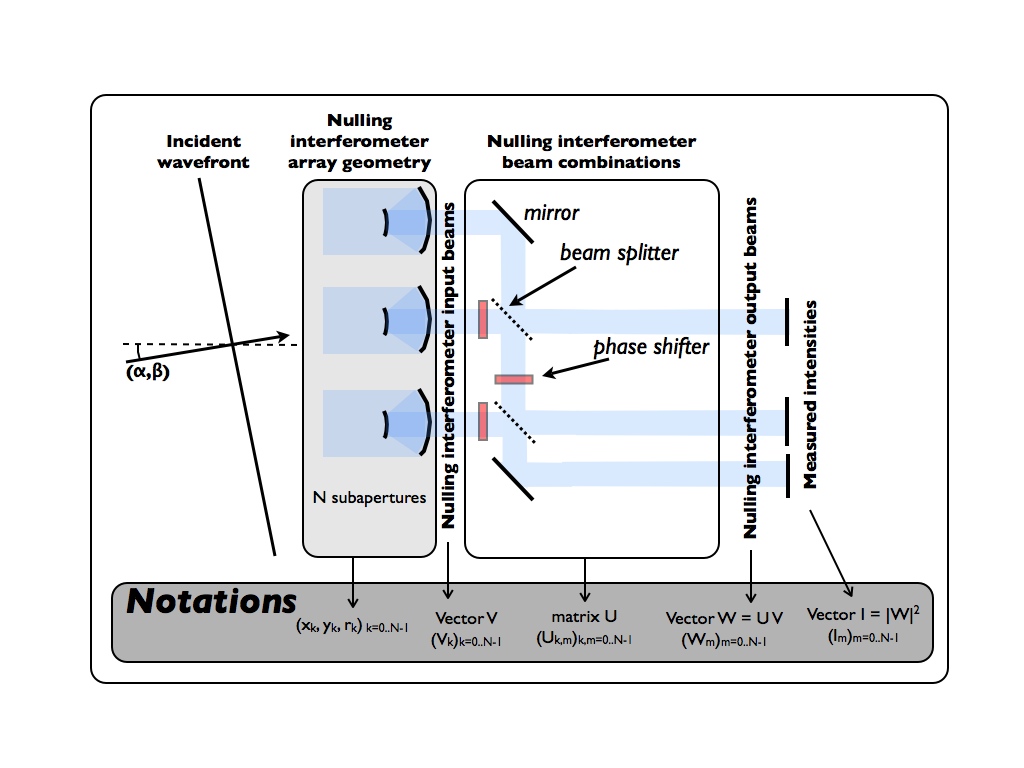Fig 1: Notations used. The indices used for the inputs and outputs of the interferometer's beam combination unit are n and m respectively. [jpg]

The science detector measures the square modulus I = |W|² of W. The matrix U represents the design of the nulling device, and is not a function of the input complex amplitudes V. Coefficients of U are complex numbers noted U_k,m, with k the subaperture index and m the interferometer output index. Each line U_m of U (m fixed) records the set of input complex amplitudes which, when "fed" into the interferometer, will send all of the light into interferometer output m. Since this set of inputs can generally not be written as a vector V according to equation (2.1), there may not be a position on the sky for which all light would be directed to output m (although one might choose the matrix U to send all light from a given sky position (α,β) to a single output m by setting U_m=V(α,β)). Each column U_k of U records how light from a single input k (a single subaperture) is directed to all outputs.
Since |V|² = |W|² for any input vector V (the interferometric combinations preserve total flux), U is a complex unitary matrix .

The nulling device representation adopted in this study is universal, as the matrix U can describe any coherent mixing scheme between the beams. Any matrix U can be implemented by finite numbers of beam splitters and phase shifters, but the model is not restricted to specific phase shifts or split ratios between beams, as previous studies have sometimes assumed (for example, the Laurance nulling interferometers described in Karlsson & Mennesson 2000 are limited to 0 or π phase shifts).

3. Optimal interferometric combinations for a given aperture geometry

The approach to designing an optimal interferometer, detailed in this section, is to concentrate as much starlight as possible in as few interferometer outputs as possible, therefore leaving other outputs sufficiently dark for detection of high contrast source(s). More specifically, the optimal set of interferometric combinations between the interferometer input beams is iteratively built by first directing as much of the starlight as possible in a single coherent output, therefore minimizing the total amount of starlight in all other outputs. The beam combinations between the remaining outputs are then optimized to maximize residual starlight is a single coherent output, and so on. This iterative approach ensures that, provided that the interferometer output beams are ranked in decreasing order with amount of residual starlight, the amount of starlight in each output is optimally minimal. The resulting interferometer design will maximize planet detection SNR, as it will provide as many nulled outputs as possible, therefore simultaneously optimizing null depth and throughput. This approach is different from only optimizing null depth, which may lead to a design for which a single output is nulled while all other outputs retain a significant amount of starlight - a solution which would offer a low efficiency for planet detection. Another advantage of this approach is that the optimal nulling device design (matrix U) is largely independent of target parameters (value of stellar angular size, planet to star position or contrast), and is only a function of the array geometry, as discussed in this section.

3.1. Unresolved central source (rs = 0)

3.2. Partially resolved central source (rs > 0)

If the central source is partially resolved, it is no longer described as a single vector V, but as a set of NBpt vectors V_pt = V(α_pt,β_pt) with α_pt and β_pt (pt = 0 .. NBpt-1) uniformly distributed over the stellar radius. The measured intensities at the output of the interferometer are obtained by summing incoherently the intensity vectors for each of the points on the stellar surface.

I(star) = (1/NBpt) x ∑pt=0..NBptIpt = (1/NBpt) x ∑pt=0..NBpt |U V(αpt,βpt)|2	(3.1)

The optimal set of interferometric combinations (defined by the matrix U) is the one that concentrates the most starlight in the smallest number of outputs. While it is no longer possible to concentrate all starlight in a single output, it is possible to identify the values of the coefficients on the first line U_m=0 of U which maximizes the amount of starlight in the first output (m=0) of the interferometer. A small amount of residual starlight is then spread over the other outputs (m=1..N-1) according to the other lines of U. The second line U_m=1 of U can be chosen to concentrate as much as this residual starlight on output m=1. This process is repeated N times until the full matrix U is built. This iterative process ensures that the stellar flux decreases as rapidly as possible as the interferometer output number increases.

Mathematically, the operations described above is a Principal Components Analysis (PCA), which can be performed by singular value decomposition of the NBpt-by-N transpose A of the data matrix A^T. A is composed of the vectors V_pt (each column pt of the matrix A is the vector V_pt=V(α_pt,β_pt)):

A = U Σ B*	(3.2a)

where U is a N-by-N complex unitary matrix, Σ is a N-by-NBpt matrix containing the singular values of A ordered in decreasing amplitude, and B is a NBpt-by-NBpt matrix. The PCA decomposition Y^T of the data matrix A^T is given by:

YT = AT U	(3.2b)

The columns of the matrix U are the principal components vectors, ordered in decreasing order of amplitude. The fist column of U is the first principal component: it is a unity norm vector which represent the dominant variability (maximum variance) in the data set composed of the vectors V_pt. The second column of U is the second principal component: it is also a unity vector, orthogonal to the first principal component vector, which represents the dominant variability in the data set after removal of the first principal component contribution in the data.

3.3. Interferometer modal response to finite angular stellar diameter

The SVD operation described above identifies and sorts the dominant "modes" U_m (m=0..N-1) present in the set of NBpt vectors V_pt used to model the star, and builds the interferometric combinations which link each of these modes to a single output of the interferometer. The first mode U_m=0 is equal to the vector V(0,0) and has a singular value close to 1 (strictly equal to 1 if the star has a radius rs = 0), and subsequent singular values are much smaller unless rs becomes comparable to the interferometer's diffraction limit.

In a randomly chosen 2-D interferometer with a stellar size smaller than the interferometer's diffraction limit, the second and third modes are 2nd order modes of stellar size: their intensity (square of amplitude) contribution to a vector V(α,β) increases as a linear combination of α² and β². The next 3 modes are 4rth order, and the following 4 modes are 6th order.
This property is a direct consequence of the Taylor expansion of equation (2.1):

ei(αx+βy) = 1 + iαx + iβy - (1/2)(α2x2 + 2αβxy + β2y2) - (i/6)(α3x3 - 3α2βx2y - 3αβ2xy2 - β3y3) + ....	(3.3)

This expansion, when inserted into equation (3.1), produces a single 0th order mode, two 2nd order modes, three 4th order modes, followed by modes of 6th order or higher. For rs smaller than the interferometer diffraction limit, these modes correspond to the interferometer outputs when the beam combiner is optimally design: output m=0 is the bright 0th-order mode where most of the starlight is directed, outputs m=1,2 are the 2nd order modes (light in these outputs of the interferometer increases as the square of stellar size), outputs m=3,4,5 are the 4th order modes, and so on up to the number of subapertures (= number of outputs). The expected correspondence between the modes obtained by Taylor expansion and the modes produces by the SVD is physically due to the very rapid decrease of starlight present in the Taylor expansion modes as a function of mode order. For a small angular radius star, the optimal way to concentrate light in a single interferometric output is to match this output with the 0-th order mode obtained by the Taylor expansion. The next optimal two modes should then be matched to the 2nd order modes in the Taylor expansion, and so on.

3.4. Important predictions

PREDICTION 1: In a 2-D interferometer of N subapertures, the minimum achievable null depth γ is γ=2 for N=2,3, γ=4 for N=4,5,6, γ=6 for N=7,8,9,10. For any aperture geometry, there exists a coherent mixing of the beams that will reach this null depth using a finite number of beam splitters and phase shifters.

The proof for this prediction is given in section 3.3., where it is shown that a SVD decomposition can be used to design the interferometer nulling device reaching the null depth stated above. The performance of 2-D nulling interferometers is therefore not a smooth function of number of apertures N when performance is limited by stellar angular size. Increasing the number of apertures from N=5 to N=6 does not bring a large increase in performance, while going from N=6 to N=7 does by allowing a 6-th order null.

PREDICTION 2: For the same number of apertures N equal or greater than 3, 1-D interferometers can reach deeper null than 2-D interferometers.

The analysis in section 3.3 shows that at high contrast, the key to designing a high sensitivity interferometer with a limited number of apertures is to remove the number of relevant low order terms (=make the coefficient in front of the term very small) in equation (3.3) to rapidly gain access to higher order modes without having to increase the number of subapertures. This can best be done with a 1-D interferometer, where the Taylor expansion becomes:

ei(αx) = 1 + iαx - α2x2/2 - iα3x3/6 + ....	(3.4)

In any 1-D interferometer, starlight on the interferometer output m (numbered from 0 to N-1) therefore increases as the 2m power of stellar angular size, allowing deeper null than a 2-D interferometer with the same number of apertures. Table 1, gives the minimum null depth achievable as a function of number of apertures in 1-D and 2-D, according to the SVD analysis and Taylor expansion presented in section 3.3. For the same number of apertures, considerably deeper nulls can be achieved with 1-D geometry than can be achieved with a 2-D geometry. For example, any 1-D interferometer geometry can provide a 6th order null with only 4 apertures, while a randomly chosen 2-D geometry would require 7 apertures. With a small number of subapertures, it is thus expected that 1-D or quasi 1-D geometry will be preferred when stellar angular size drives the interferometer's sensitivity.

Previously published interferometer designs illustrate the fundamental advantage of 1-D arrays for null depth, and many previously suggested interferometer designs reach the minimum achievable null depth shown in table 1. The Angel Cross design [Angel 1990] is a 2-D geometry to achieving a θ⁴ null, while a linear array with the same number of apertures can offer a θ⁶ [ Angel & Woolf 1997 ]. The 2-D 6-aperture Mariotti configuration [Mennesson et al. 2005] achieves a θ⁴ null. Collapsing the 4-aperture 2-D Angel cross geometry into a 3-aperture 1-D array yields the degenerate Angel cross, with a θ⁴ null. The best reported null depth with small number of apertures are indeed 1-D geometries, and reach the limits shown in table 1: θ⁶ null with 4 apertures [ Angel & Woolf 1997 ] and θ⁸ null with 5 apertures [Woolf & Angel 1997].

Rouan 2006 proposes a method to design 1-D nulling interferometer designs offering a θ^2L null with 2^L apertures. The iterative method employed to do so is simple and showed for the first time that arbitrarily deep nulls can be achieved given a sufficient number of apertures. As shown by table 1, it is however not optimal, as a θ^2L null can be obtained with any set of L+1 apertures.

PREDICTION 3: Interferometer effective throughput increases with number of apertures

PREDICTION 4: The optimal nulling coherent beam combiner only uses phase shifts equals to 0 and π

4. Interferometer designs

4.1. Linear arrays

4.1.1. Angel & Woolf 4-aperture design

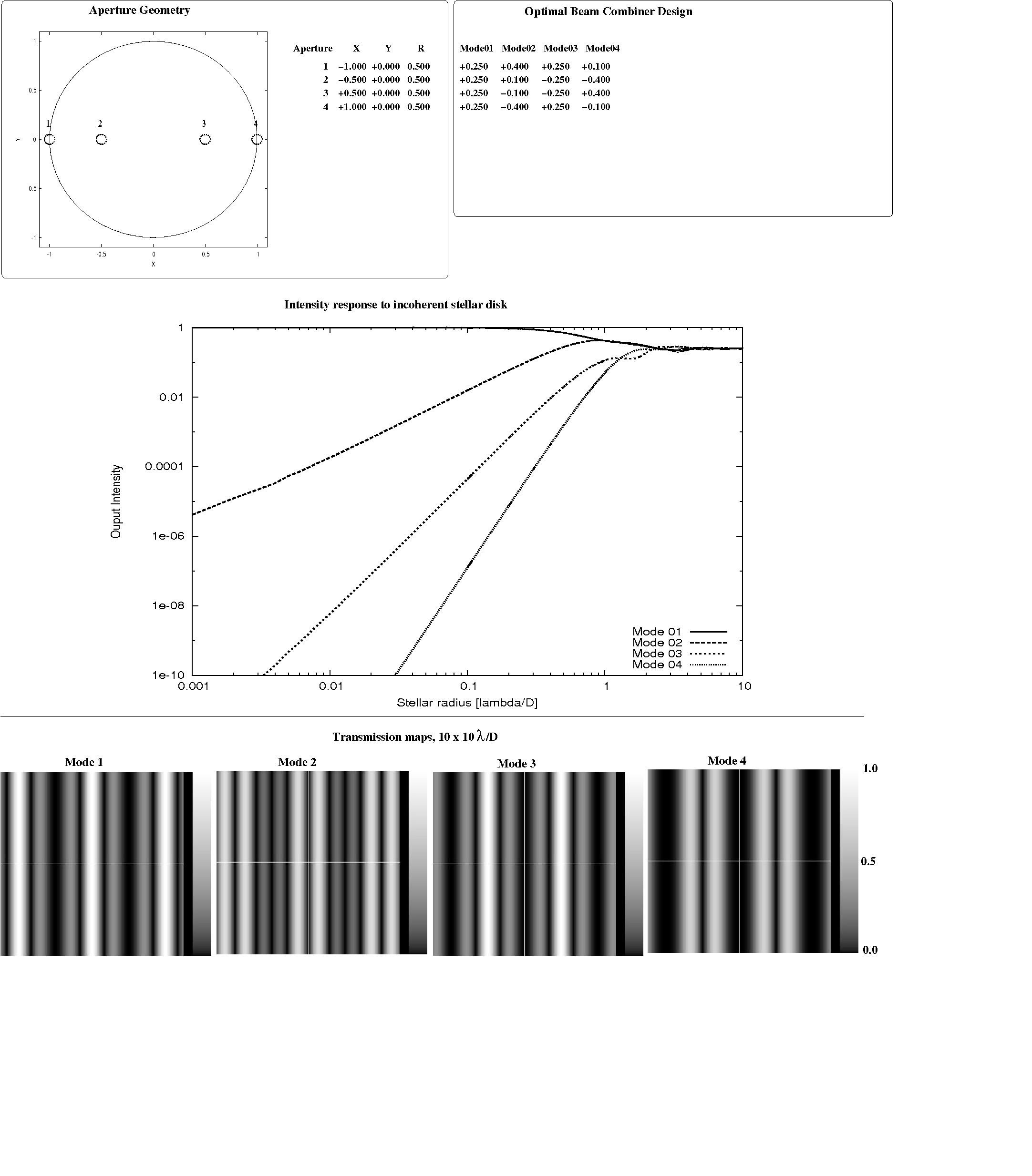Fig 4.1: Beam combiner solution for the linear 4-aperture geometry proposed in Angel & Woolf 1997. The aperture geometry is shown in the upper left. The optimal beam combiner design, as obtained by the SVD approach described in this paper is shown in the upper right table, where each column corresponds to one interferometer output, and the coefficients of the table show how each aperture (lines of the table) is split between the outputs. The element (i,j) of the table indicates the fraction of the intensity collected by aperture (i) that is directed to interferometer output (j), and a negative value indicates a π phase shift. The distribution of light intensity among the four outputs for the observation of an incoherent stellar disk is shown in the plot at the center of the figure, as a function of stellar angular radius (x-axis). The intensity transmission map for each of the four interferometer outputs is shown in the lower part of the figure. [eps]

The first output of the interferometer (Mode 1 in figure 4.1) contains most of the starlight, while modes 2, 3 and 4 show respectively θ², θ⁴, and θ⁶ intensity dependence with stellar angular size. The ability to produce a 6th order null with this 4-aperture geometry, first described by Angel & Woolf 1997, is thus confirmed by the SVD analysis. The beam combinations that produce this deep null, as given by the SVD (last column of the table at the upper right of figure 1) also match the combination identified by Angel and Woolf: the dark output of the inner 2-aperture Bracewell interferometer (apertures 2 and 3, coefficients -0.4, 0.4) is combined with the dark output of the outer Bracewell interferometer (apertures 1 and 4, coefficients 0.1, -0.1). As Angel and Woolf described, the two Bracewell interferometers have opposite signs, and the inner interferometer is given 4 times (2 times in amplitude) the weight of the the outer interferometer. The solution given by the SVD analysis offers superior sensitivity to the beam combiner design proposed in Angel & Woolf 1997 , as it also offers a θ² null (output 2) and a θ⁴ null (output 3), while the beam combining configuration proposed in Angel & Woolf 1997 offered two bright outputs (O1 and O2 in fig 1 of their paper) and a single θ² output (O3 in fig 1 of their paper). This could be achieved by recombining together outputs O1, O2 and O3 of the beam combiner shown in fig 1 of Angel & Woolf 1997 according to the values given in the table at the upper right of figure 4.1.

Angel & Woolf 1997 suggested sightly increasing the amplitude of the outer Bracewell pair relative to the inner pair to achieve a wider null, suggesting a 0.504 relative ratio in amplitude (as opposed to 0.5 in the design described above). The effect of doing so on the null depth is shown in fig 2 of their paper, where three local minima in output intensity are shown within the null, located at approximately -0.1 λ/B, 0 and +0.1 λ/B. To explore this possibility, the SVD analysis is repeated on the same interferometer geometry, but with an 0.1 λ/B stellar radius. Results, shown in figure 4.2., not only confirm that increasing the relative weight of the outer apertures increases null depth, but demonstrate that doing so is the optimal solution to the nulling beam combiner design. The optimal value for the relative weight in amplitude should be sqrt(0.10097/0.39903) = 0.503 for a 0.1 λ/B radius stellar disk, close to the 0.504 value proposed by Angel & Woolf, and the transmission map has 3 local minima at -0.8 λ/B, 0 and +0.8 λ/B, as shown by the local minimum of the intensity output curve vs. stellar diameter for mode 4 in figure 4.2.

Fig 4.2: Optimal beam combiner solution for the linear 4-aperture geometry proposed in Angel & Woolf 1997, computed here for a 0.1 λ/B stellar radius. The solution differs from the small stellar size limit (figure 4.1) in the same way as predicted in Angel & Woolf 1997: more weight should be given to outer apertures in the deepest null output. [eps]

4.1.2. Optimal beam combiner design for arbitrary linear geometries

A key result of the SVD-based construction of optimal beam combiners for nulling interferometers is the ability to produce deep nulls regardless of aperture geometry. The technique predicts for example that θ⁶ and θ⁸ nulls can be constructed out of respectively any 4-aperture linear array and any 5-aperture linear array.

Figure 4.3 shows the result of the SVD-based technique for a randomly chosen 5-aperture linear array geometry. The θ⁸ deep null produced is especially resilient to stellar angular size and pointing errors: its transmission for a 0.1 λ/B radius disk is below 1e-10. For this randomly chosen geometry, the beam mixing ratios producing the deep null are non-trivial values, with no recognizable integer ratio between the contributions of entrance apertures. The optimal solution also offers other nulled outputs, with nulled orders of respectively 2, 4 and 6, in agreement with the small stellar size limit analysis presented in section 3.

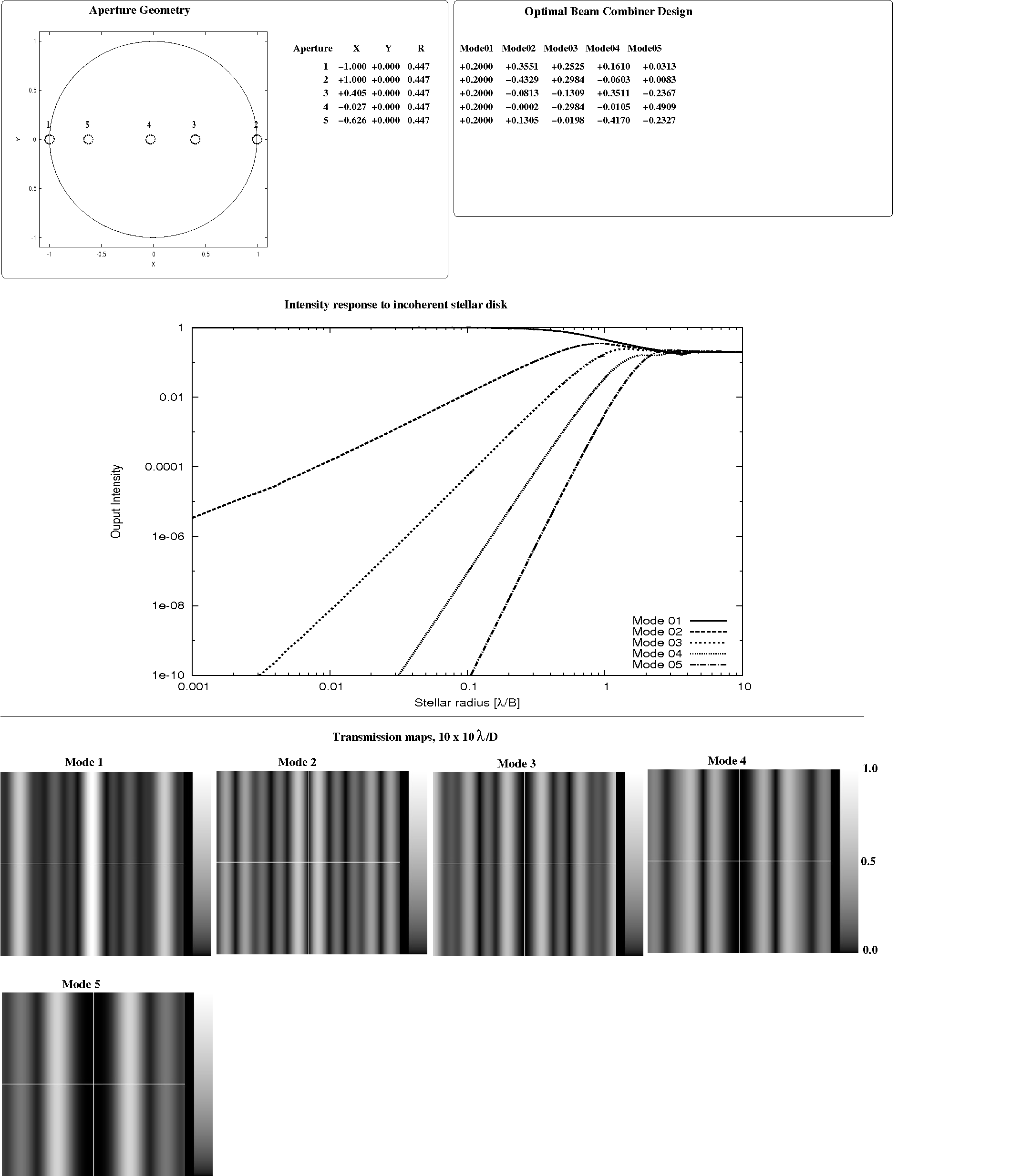Fig 4.3: Optimal beam combiner solution for a randomly chosen linear 5-aperture geometry, computed here for a 0.001 λ/B stellar radius. As predicted in section 3, the solution produces an output with a deep θ8 null, along with 3 other nulled outputs offering θ6, θ4 and θ2 deep nulls. [eps]

The ability to produce deep nulls regardless of aperture geometry allows high performance nulling interferometry to be carried on an array geometry optimized for (u,v) plane coverage. Figure 4.4 shows the array geometry and beam combiner design for a 4-aperture array optimized for single-dimension (u,v) plane coverage. The baselines covered by this array are all the (kB/6), with k=1..6, allowing excellent (u,v) plane coverage if the array is rotated around the line of sight. The SVD-based technique does produce a θ⁶ deep null, along with two other nulls of order 2 and 4 respectively.

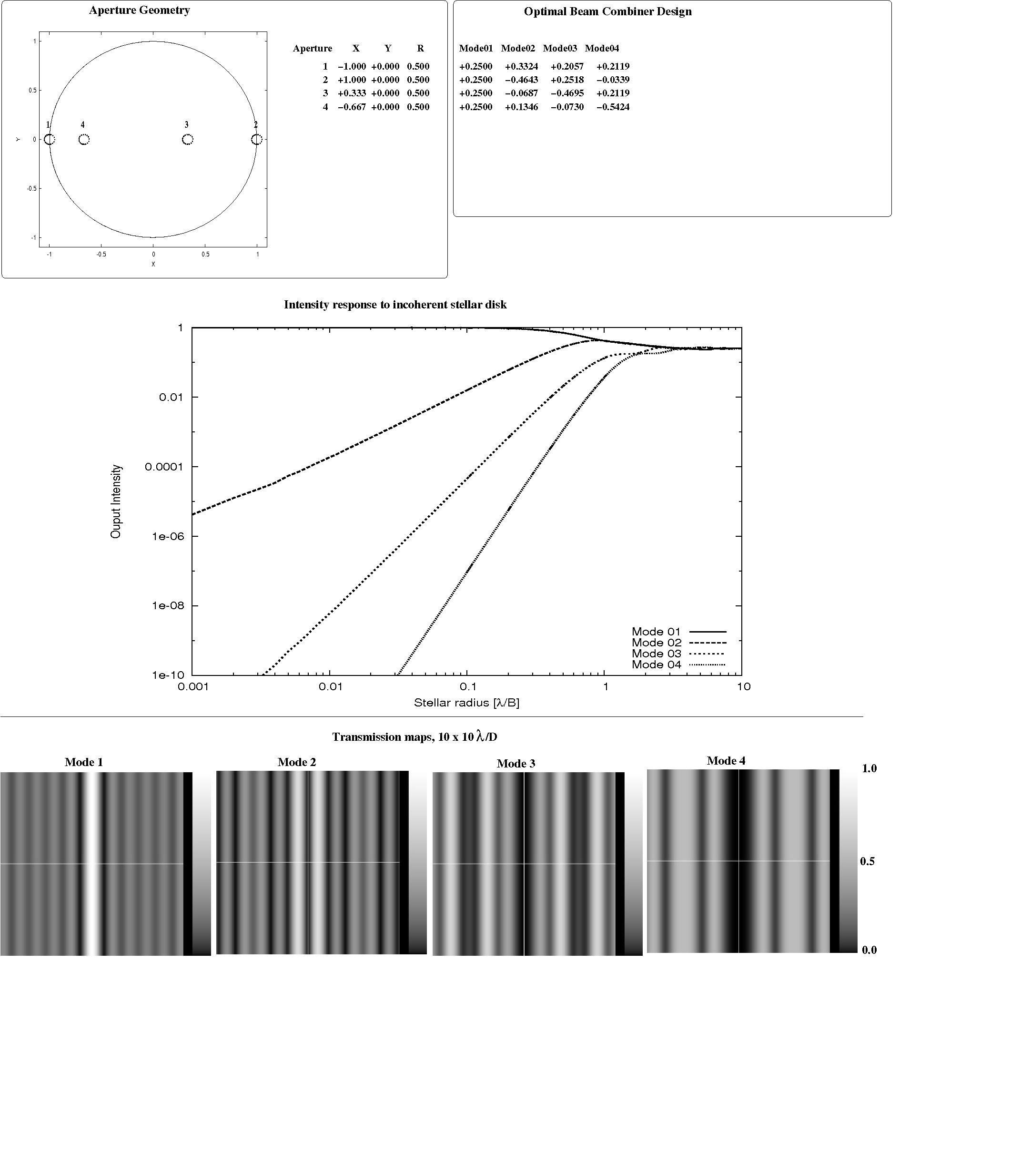Fig 4.4: Optimal beam combiner solution for a linear 4-aperture array geometry optimized for (u,v) plane coverage, computed here for a 0.001 λ/B stellar radius. As predicted in section 3, the solution produces an output with a deep θ6 null, along with 2 other nulled outputs offering θ4 and θ2 deep nulls. [eps]

4.2. 2-D arrays

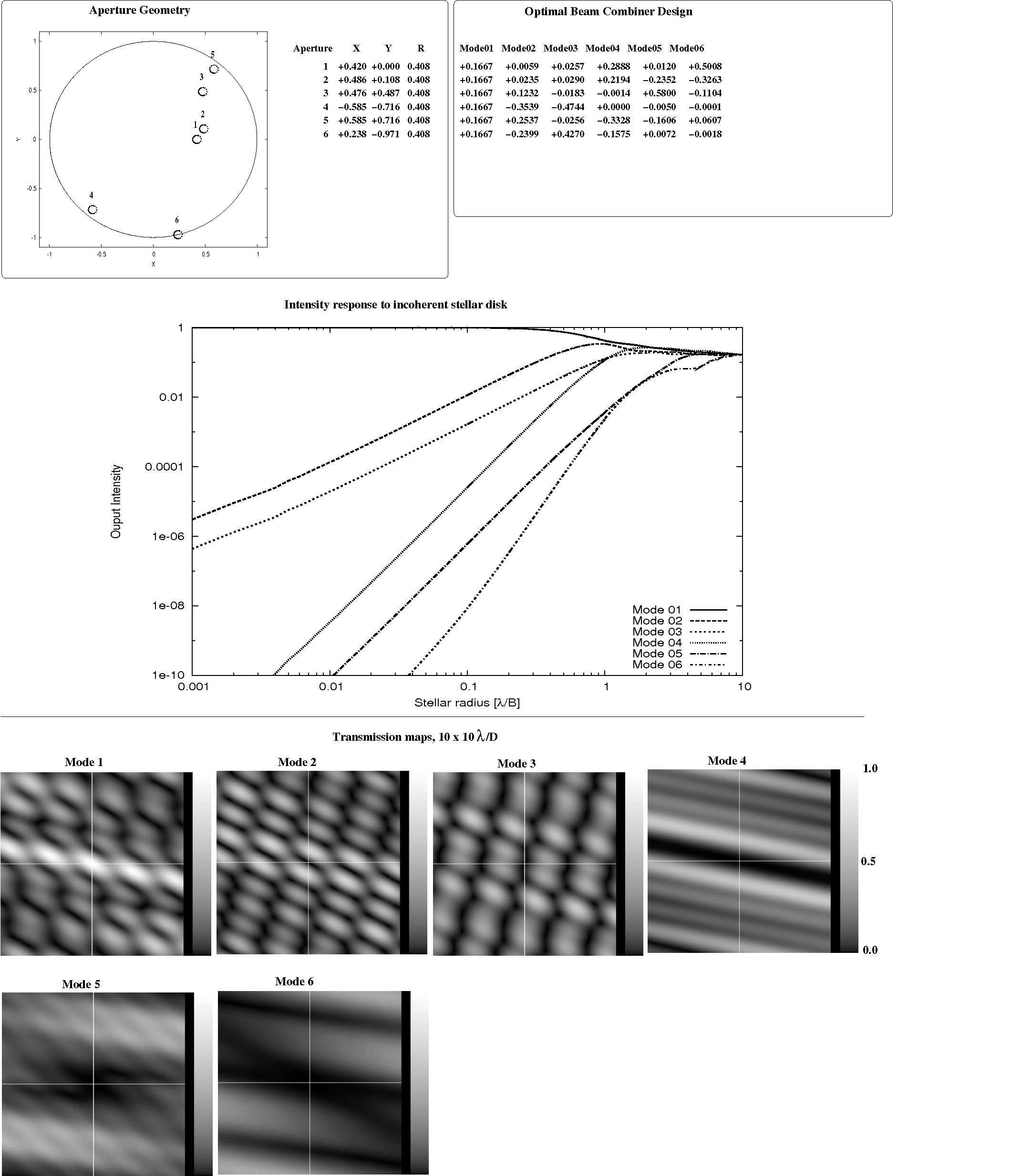Fig 4.5: Optimal beam combiner solution for a 2-D 6-aperture array geometry optimized for (u,v) plane coverage, computed here for a 0.001 λ/B stellar radius. As predicted in section 3, the solution produces three outputs with a deep θ4 null, along with 2 other nulled outputs offering θ2 deep nulls. [eps]

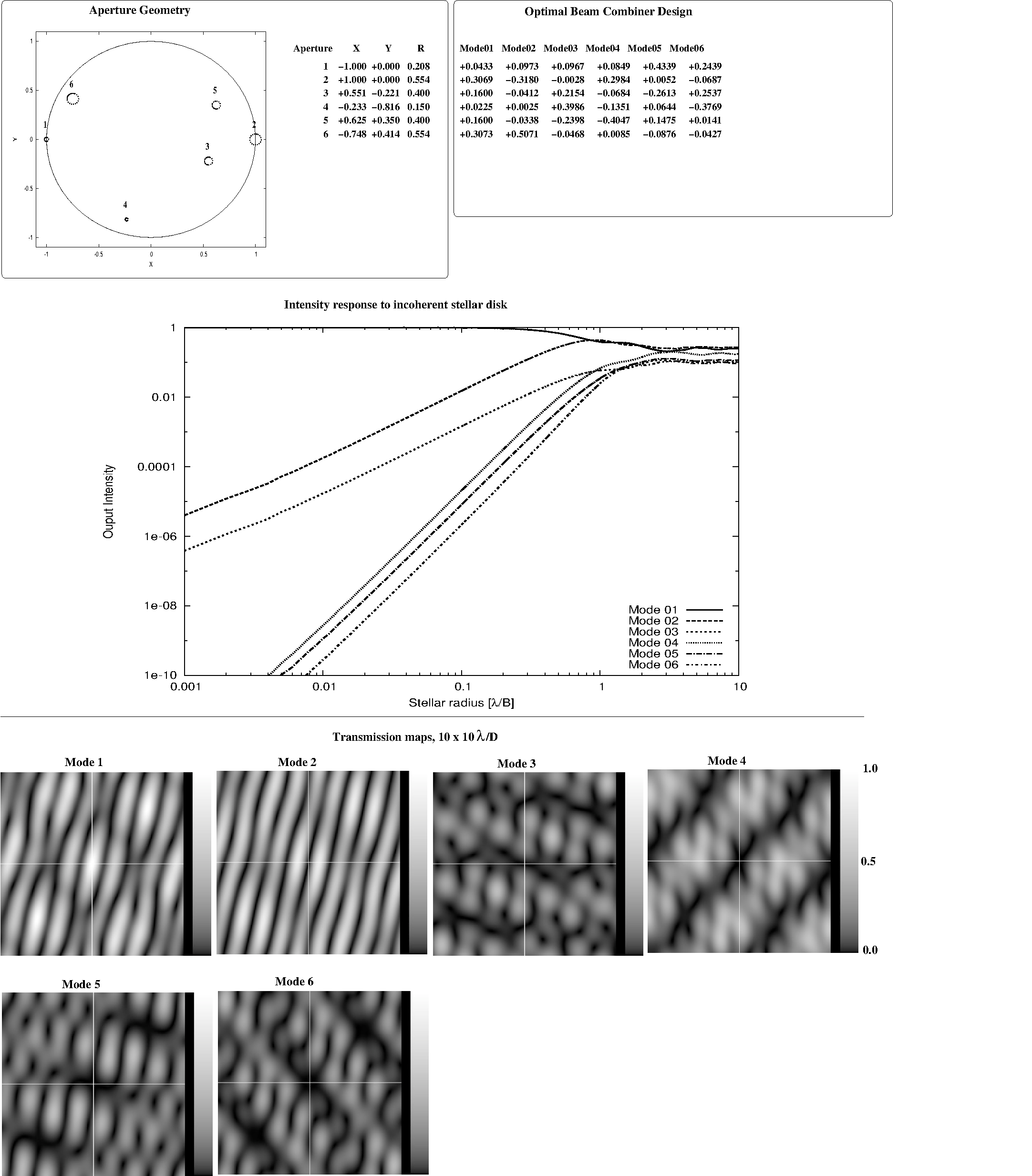Fig 4.6: Optimal beam combiner solution for a 6-aperture array geometry for which the subaperture positions and sizes were randomly chosen. The solution was computed for a 0.001 λ/B stellar radius. As predicted in section 3, the solution produces three outputs with a deep θ4 null, along with 2 other nulled outputs offering θ2 deep nulls. [eps]

Conclusion

The analysis performed in this paper shows that null depth in a nulling interferometer is primarily a function of the number of apertures, and that nulls of sufficient depth to detect and characterize exoplanets can be achieved with relatively small number of apertures (4 to 10), regardless of geometry. The superiority of 1-D arrays for achieving deep nulls with a small number of apertures, a trend that is strongly supported by previously published nulling interferometer designs, has been demonstrated and quantified. The SVD-based approach introduced in this paper allows optimal design of beam combiners for nulling interferometry, and is highly flexible, as it can be applied to any geometry, and can also optimally take into account stellar angular size.

While the SVD-based technique has been used to derive the minimal null depth achievable as a function of number of apertures, no strict limit has been placed on the maximum null depth achievable as a function of number of apertures. Specific array geometries may allow deeper nulls than the lower limits shown in table 1, which would enable cost-effective nulling interferometer consisting of very few apertures to be implemented for imaging and spectral characterization of exoplanets.

While the beam combining design in this paper are entirely driven by null depth for a finite stellar angular size, additional considerations must be taken into account in the design of a nulling interferometer, such as sensitivity to background light (especially important at long wavelength, for which zodiacal background exceeds planet light contribution), imaging performance, and resilience to cophasing errors. The impact of exozodiacal light was not considered in this study, but may also drive the optimal array geometry [Defrere et al 2010] and beam combining scheme. These additional constraints should be combined into the SVD-based analysis presented in this paper.

Additional References, links

• Olivier Absil's paper on nulling interferometer configurations