
[eps]
The unprecedented angular resolution soon to be offered by extremely large telescopes (ELTs), together with recently developed high contrast imaging techniques (coronagraphy and wavefront control), will enable direct imaging and spectroscopic characterization of potentially habitable planets around nearby M-type stars. While the habitable zones of M stars is challenging to resolve, the planet to star contrast and the apparent brightness of the planet are highly favorable, thus providing the only reliable opportunity for direct imaging and spectroscopic characterization of habitable planets from the ground.
The key to imaging and characterizing such planets lies in the ability to perform high contrast imaging (approximately 1e-5 raw contrast) at $\approx$ 1 λ/D with high photometric efficiency. Technical solutions to this challenge now exist, as illustrated by the recent development of a full throughput coronagraph concept offering sub-λ/D inner working angle at high contrast on segmented apertures, and schemes to achieve the necessary level of pointing and low order wavefront error control. Demonstrations of these key techniques are ongoing in laboratories and on ground-based telescopes, already yielding encouraging results. We conclude that a highly specialized, but relatively simple, high contrast imaging system can be build for ELTs within this decade, and that it would likely provide the first opportunity to acquire high quality spectra of habitable planets, before space-based telescope can provide similar capabilities for brighter F-G-K type stars.
Characterization of potential habitable planets around other stars to the level required for identification of biological activity requires relatively high quality spectroscopy.
In Section 2, the expected first-order observational characteristics (planet contrast, separation and apparent luminosity; star brightness) of rocky planets in the habitable zones of nearby stars are established. Using these parameters, section 3 shows that rocky planets around M-type stars can be observed with ELTs in reflected light provided that (1) a coronagraph operating with a 1 λ/D inner working angle can be used and (2) wavefront sensing can be performed efficiently on low-order aberrations. These two requirements are then discussed in more detail in sections 4 (coronagraphy) and 5 (wavefront control and calibration).
Blue fit (B-V < 1.2):
fitblue(x) = ab + bb*x + cb*x**2 + db*x**3

degrees of freedom    (FIT_NDF)                        : 20
rms of residuals      (FIT_STDFIT) = sqrt(WSSR/ndf)    : 0.0321603
variance of residuals (reduced chisquare) = WSSR/ndf   : 0.00103429

Final set of parameters            Asymptotic Standard Error
=======================            ==========================

ab              = -0.121112        +/- 0.03043      (25.12%)
bb              = 0.634846         +/- 0.2317       (36.5%)
cb              = -1.01318         +/- 0.4267       (42.12%)
db              = 0.125024         +/- 0.217        (173.6%)
Red fit (B-V > 1.0):
fitred(x) = ar + br*x + cr*x**2 + dr*x**3 + er*x**4

degrees of freedom    (FIT_NDF)                        : 73
rms of residuals      (FIT_STDFIT) = sqrt(WSSR/ndf)    : 0.250859
variance of residuals (reduced chisquare) = WSSR/ndf   : 0.0629302

Final set of parameters            Asymptotic Standard Error
=======================            ==========================

ar               = -43.9614         +/- 20.91        (47.56%)
br               = 115.958          +/- 54.3         (46.83%)
cr               = -110.511         +/- 51.86        (46.93%)
dr               = 44.7847          +/- 21.63        (48.29%)
er               = -6.74903         +/- 3.327        (49.29%)
| |
Fig 1: Bolometric correction as a function of B-V color for the 8-pc sample. The blue and red fits are used for B-V < 1.1 and B-V > 1.1 respectively. [eps] |
The bolometric luminosity (referenced to the Sun) for each star is then derived from the absolute magnitude MV and the bolometric correction BC():
| Lbol = 2.51188643-(MV-4.83) + (BC - BCSun) | (1) |
|---|
The planet is then placed sqrt(Lbol) AU from the star, and its angular separation is computed using the star parallax.
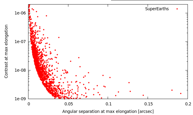 |
Fig 2: Angular separation vs reflected light contrast for SuperEarths (2x Earth diameter), assuming each star in the sample has such a planet. [eps] |
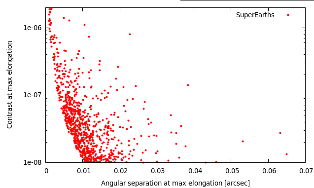 |
Fig 3: Angular separation vs reflected light contrast for SuperEarths (2x Earth diameter), assuming each star in the sample has such a planet (detail). [eps] |
degrees of freedom    (FIT_NDF)                        : 76
rms of residuals      (FIT_STDFIT) = sqrt(WSSR/ndf)    : 0.0741659
variance of residuals (reduced chisquare) = WSSR/ndf   : 0.00550058

Final set of parameters            Asymptotic Standard Error
=======================            ==========================

a               = 0.0207711        +/- 0.07513      (361.7%)
b               = 0.571443         +/- 0.233        (40.78%)
c               = -0.157074        +/- 0.2176       (138.5%)
d               = 0.147305         +/- 0.06183      (41.97%)
V-I fit as a function of B-V:
degrees of freedom    (FIT_NDF)                        : 76
rms of residuals      (FIT_STDFIT) = sqrt(WSSR/ndf)    : 0.1921
variance of residuals (reduced chisquare) = WSSR/ndf   : 0.0369025

Final set of parameters            Asymptotic Standard Error
=======================            ==========================

a               = 0.221522         +/- 0.1946       (87.84%)
b               = 0.0067191        +/- 0.6036       (8984%)
c               = 0.906601         +/- 0.5636       (62.17%)
d               = 0.000695602      +/- 0.1601       (2.302e+04%)
This study assumes that planet imaging is performed in the near-IR with adaptive optics. To estimate the contribution of photon noise, the near-IR brightnesses of both the stars and their planets are required
Apparent J, H and K magnitudes for the stars are extracted from the 2MASS catalog. In the few cases (1% of the targets) where Gliese catalog entries do not have a match in the 2MASS catalog (usually because they are too faint or they are close companions), 4th order polynomial fits of the V-J, V-H and V-K colors as a function of B-V color are derived from the list of targets that are matched in both catalogs, and then applied to those for which no near-IR flux measurement exists. In this case, the standard deviation in the J, H, and K magnitudes are 0.36, 0.41 and 0.36 respectively (these values are sufficiently small to not significantly affect planet detectability estimates).
Since the planet albedo is assumed independent of wavelength, the planet to star contrast in the near-IR is the same as computed for visible light. No thermal emission is assumed (this is a conservative assumption in K band).
These detectability constraints are highly coupled. For example, the contrast limit is usually a steep function of the angular separation, and both the star brightness and planet brightness strongly affect the contrast limit. The interdependencies between these limits are function of the instrument design and choices (wavefront control techniques, observation wavelength). To easily identify how instrumental trades affect detectability of habitable exoplanets, first cut limits are first applied to construct a small list of potential targets.
| Limit/constraints | Comments | |
|---|---|---|
| Angular Separation | Must be > 1.0 λ/D | Limit imposed by coronagraph (see section 4). Corresponds to 11mas on a 30-m telescope in H band. |
| Contrast | Must be > 1e-8 | High contrast imaging limit (see section 5) |
| Star brightness | Must be brighter than mR = 15 | Required for high efficiency wavefront correction (see section 5) |
| Planet Brightness | Must be brighter than mH = 26.8 | Faint detection limit |
The first cut limits are shown in the table above. The number of targets kept is mostly driven by the contrast and separation limits, and to a lesser extent by the planet brightness limit. The planet brightness limit is derived from a required SNR=10 detection in 10mn exposure in a 0.05 μm wide effective bandwidth (equivalent to a 15% efficiency for the whole H-band) on a 30-m diffraction limited telescope, taking into account only sky background and assuming all flux in a 20mas wide box is summed. The assumed sky background (continuum + emission) is mH = 14.4 mag/arcsec2 [E-ELT sky background model, ESO] and [Cuby et al. 2000].
D=30 -> 700 m2
background = 16412 ph / sec / um / m2 / arcsec2 -> 230 ph/sec on the 20mas box
With N photon/sec from source: SNR(t) = N sqrt(t) / sqrt(N + 230)
With t = 600 sec -> SNR = 24.5 N / sqrt(N+230)
SNR = 10 ->  N = 6.3 ph/sec
flux = 6.3 ph/sec = 0.18 ph/sec/um/m2 -> mH = 26.8
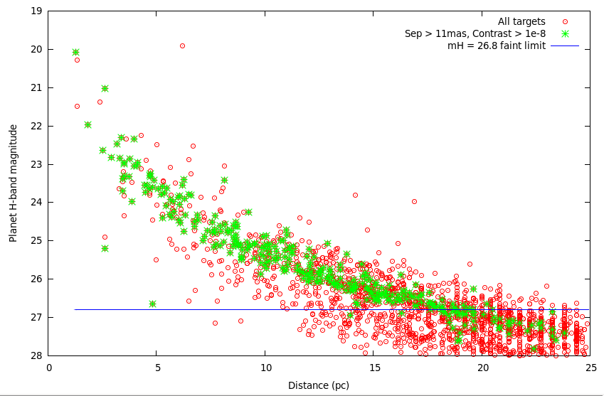 |
Fig 4: Planet apparent brightness in H-band as a function of system distance. The mH=26.8 flux limit adopted excludes planets beyond 20pc.plot [0:20][28:19] "./cat1.dat" u 1:($26-2.5*log10($10)) w p ps 0.4 pt 7[eps] |
The target list after applying the first cut limit consists of 274 entries. Figure x shows that this lists consists mostly of relatively faint (mV~10) late-type (V-R ~ 1 to 1.5) main sequence stars. Two notable exceptions are the 40 Eri B and Sirius B white dwarfs, clearly visible in fig x as much bluer (V-R ~ 0) than the rest of the sample.
 |
Fig 5: ELT exoplanet targets stars visible light brightness and color. [eps] |
| STAR | PLANET | ||||||||||
|---|---|---|---|---|---|---|---|---|---|---|---|
| Name | Type | Distance | Diameter | Lbol | mV | mR | mH | Separation | Contrast | mH | Notes, Multiplicity |
| Proxima Centauri (Gl551) | M5.5 | 1.30 pc | 0.138 RSun 0.990 +- 0.050 mas [1] | 8.64e-04 | 11.00 | 9.56 | 4.83 | 22.69 mas | 8.05e-07 | 20.07 | RV measurement exclude planet above 3 Earth mass in HZ [Endl & Kurster 2008] |
| Barnard's Star (Gl699) | M4 | 1.83 pc | 0.193 RSun 0.987 += 0.04 mas [2] | 4.96e-03 | 9.50 | 8.18 | 4.83 | 38.41 mas | 1.40e-07 | 21.97 | - |
| Kruger 60 B (Gl860B) | M4 | 3.97 pc | 0.2 RSun[3] | 5.81e-03 | 11.30 | 9.90 | 5.04 | 19.20 mas | 1.20e-07 | 22.35 | - |
| Ross 154 (Gl729) | M4.5 | 2.93 pc | 0.2 RSun[3] | 5.09e-03 | 10.40 | 9.11 | 5.66 | 24.34 mas | 1.37e-07 | 22.82 | - |
| Ross 128 (Gl447) | M4.5 | 3.32 pc | 0.2 RSun[3] | 3.98e-03 | 11.10 | 9.77 | 5.95 | 18.99 mas | 1.75e-07 | 22.84 | - |
| Ross 614 A (Gl234A) | M4.5 | 4.13 pc | 0.2 RSun[3] | 5.23e-03 | 11.10 | 9.82 | 5.75 | 17.51 mas | 1.33e-07 | 22.95 | Double star (sep=3.8 AU) |
| Gl682 | M3.5 | 4.73 pc | 0.26 RSun[3] | 6.41e-03 | 10.90 | 9.70 | 5.92 | 16.93 mas | 1.09e-07 | 23.33 | - |
| Groombridge 34 B (Gl15B) | M6 | 3.45 pc | 0.18 RSun[3] | 5.25e-03 | 11.00 | 9.61 | 6.19 | 20.98 mas | 1.33e-07 | 23.39 | 150 AU from M2 primary |
| 40 Eri C (Gl166C) | M4.5 | 4.83 pc | 0.23 RSun[3] | 5.92e-03 | 11.10 | 9.88 | 6.28 | 15.93 mas | 1.18e-07 | 23.61 | 35AU from 40 Eri B (white dwarf), 420 AU from 40 Eri A (K1) |
| GJ 3379 | M4 | 5.37 pc | 0.24 RSun[3] | 6.56e-03 | 11.30 | 10.06 | 6.31 | 15.09 mas | 1.06e-07 | 23.75 | - |
| S(λ1,λ2) = λ2/λ1 sqrt(zp1/zp2) 2.51188643(m2-m1)/2 | (2) |
|---|
| S(V,R) = 0.76 | (3) |
|---|
| S(V,I) = 0.546 | (4) |
|---|
| S(V,H) = 0.97 | (5) |
|---|
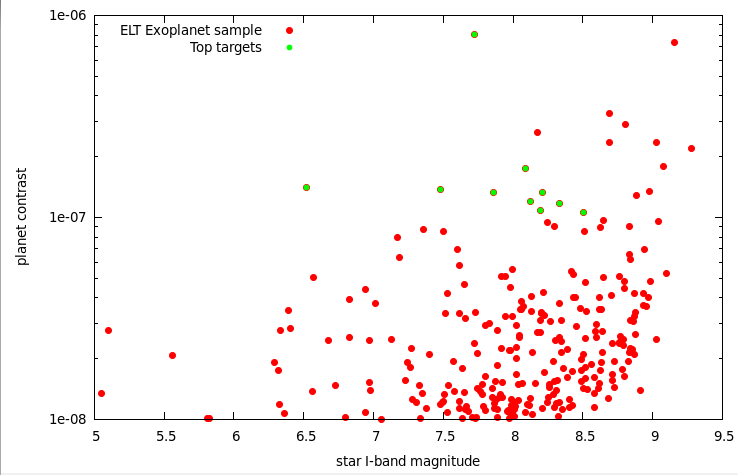 |
Fig 6: Planet contrast as a function of star I-band magnitudes for the ELT exoplanet sample and the top targets. [eps] |
The raw PSF contrast is estimated in Figure x for a mI target. In the 10 to 20 mas angular separation range where most of the exoplanets are imaged, the contrast is limited by time lag in the loop and photon noise, and the other fundamental limits to raw contrast (scintillation and atmospheric chromaticity effects) are much smaller. With a high efficiency wavefront sensor able to take advantage of the telescope's diffraction limit, the expected raw PSF contrast at these small separations is approximately 1e-5, provided that the servo lag is no more than about 0.1 ms. This unusually low servo lag can be achieved with a high WFS sampling frequency (>10 kHz), and/or the use of predictive wavefront control techniques. Figure x also shows that a seeing-limited WFS such as the SHWFS is very inefficient at these small angular separations, and would be a poor choice for the system, even if it operates at its photon-noise limit with no loop servo lag other than the one imposed by photon noise.
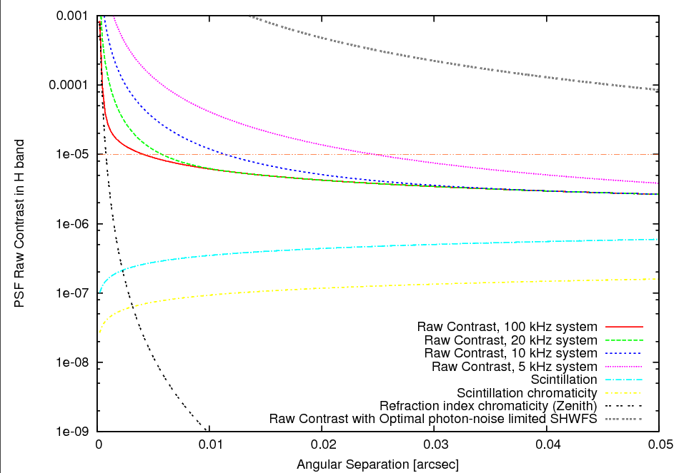 |
Fig 7: Raw contrast in a Extreme-AO corrected PSF on a 30-m telescope. The WFS is assumed to be operating at the diffraction limited sensitivity on a mI=8.5 target, with a 0.05 μm effective spectral bandwidth. For comparison, the photon-noise limited raw contrast limit for a SHWFS is also shown (upper curve). Several closed loop effective delays have been considered. [eps] |
The analytical model used to estimate raw contrast was also tested for an 8-m diameter telescope under the same conditions. For a 1 kHz system with a diffraction-limited wavefront sensor on an 8-m telescope, the raw contrast at 0.1" is 3e-4 (limited by servo lag), and it is 3e-5 at 0.5". These numbers are consistent with the goals of the future Extreme-AO systems on such telescopes.
The detection contrast limit is more difficult to estimate for this system, as a range of PSF calibration techniques could be used (spectral or polarimetric differentiation for example). For simplicity, it is assumed here that spectral or polarimetric PSF calibration techniques are not used, and that the detection limit is imposed by speckle structure in the long-exposure image and photon noise. It is also assumed that static and slow speckles that are not due to the atmosphere are removed by focal plane wavefront control, a scheme that has already demonstrate control and removal of static coherent speckles at the 3e-9 contrast level in the presence of much stronger dynamic speckles.
The PSF halo consists of rapid atmospheric speckles at the 1e-5 contrast level with a lifetime of no more than one millisecond (speckles of longer duration are suppressed by the AO loop). In a one-hour observation, this fast component can thus average to 5e-9 contrast assuming that the AO system has removed correlation on timescales above 1ms. In addition to these fast speckles, chromatic non-common path errors and scintillation create a speckle halo contribution at the 1e-6 contrast level. Since this component is not controlled by the AO system, its coherence time is longer, at up to about 100ms in the near-IR. A 1-hr long observation will average this component by a factor ~200, to 5e-9 contrast level. Finally, photon noise in a 1-hr exposure for a mH star and a 1e-5 raw contrast will set a 1e-9 contrast limit for a 0.05 μm effective spectral bandwidth. Combined together, the 3 effects lead to a detection contrast limit just below 1e-8 for a 1hr long exposure.
| Requirement | Technology | Performance | Maturity, Comments |
|---|---|---|---|
| Coronagraph concept | |||
| ~λ/D IWA | PIAA or PIAACMC | 0.9 λ/D IWA | 1e-6 raw contrast achieved at 1.2 λ/D in lab |
| High throughput | PIAA or PIAACMC | >99% throughput | demonstrated in lab |
| Raw contrast 1e-5 | PIAA or PIAACMC | no limit | Concept |
| 50% wide spectral band | diffractive focal plane mask | meets requirement | Design and Fabrication demonstrated, lab tests starting |
| Wavefront control - pointing | |||
| mas-level (0.1 λ/D) pointing jitter | LOWFS | sub-mas | Lab validation at 0.0003 λ/D RMS, on-sky functional test |
| 0.1 mas-level (0.01 λ/D) pointing calibration | LOWFS | <0.1 mas | Lab validation demonstrates 10x to 100x gain in contrast from LOWFS calibration signal, on-sky tests starting |
| Wavefront control | |||
| High sensitivity WFS | Pyramid, nlCWFS | diffraction-limited sensitivity | Pyr demonstrated on sky (LBT), nlCWFS under development, other options under study |
| 5 λ/D OWA | MEMS DM | 6 λ/D with 12x12 actuators | Component exists, well characterized |
| >10 kHz loop speed | fast CCD, computer, and DM | >10kHz can be achieved with current hardware | Components exist, ~20MHz pixel readout rate required is already achieved with photon-counting EMCCDs, DM response time suitable, current computer can achieve speed thanks to low actuator count |
| Calibrate/Remove slow and static speckles | Coherent mixing in focal plane | meets requirement | Demonstrated in multiple labs to 1e-8 to 1e-9 contrast, demonstrated to 3e-9 contrast limit with turbulence in lab, on-sky tests starting |
 |
Figure 8: Possible system architecture for an experiment aimed at imaging habitable planets around nearby M-type stars with an ELT.
|
Direct imaging of habitable planets around nearby M-type stars with ELTs appears to be feasible thanks to new techniques that allow high contrast imaging at small angular separation. While these planets are too close to be resolved by current telescopes, an ELT able to acquire high contrast imaging in the 10mas to 30mas separation range can image them, and their relatively high brightness would allow for spectroscopic investigations. For the top targets, Earth-size habitable exoplanet may even be detected.
The technologies required to achieve this goal exist, even though several key technologies have only recently been identified and not yet demonstrated at the required performance level in laboratories or on sky. The next decade will be extremely valuable to mature these techniques toward an integrated system that can be ready when ELTs begin science operations. Experimental systems on 8-m telescopes, such as the Subaru Coronagraphic ExtremeAO (SCExAO) instrument, are rapidly maturing the techniques proposed required for this goal, and should continue to do so through this decade. Given the unusual requirements of such a system and the relatively small number of targets, a focused instrument (more akin to a science experiment than a facility instrument) should be developed instead of a general purpose extreme-AO system similar to the current generation of ExAO systems on 8-m class telescopes. This would allow for a relatively simple system with a rapid development schedule and moderate cost - an approach that would allow ELTs to acquire the first high quality spectra of nearby M-type habitable planets. This science goal is complementary to future space mission operating in visible light, which will need to target exoplanets at more challenging contrast levels around Sun-like stars due to limited angular resolution.