Segmented apertures are an attractive technical solution for building large optical telescopes on the ground or for space. By enabling large telescope diameter, they also offer attractive performance for high contrast imaging of exoplanets and disks, thanks to the combination of fine angular resolution and large collecting area. In a previous study, it was shown that full performance coronagraphy is conceptually possible on segmented apertures, regardless of the size, number and arrangement of segments: in the absence of wavefront errors, direct imaging at high contrast (exceeding 1e10) was shown to be possible within 1 λ/D of the central source with full throughput. High contrast imaging is however very demanding in wavefront quality and stability, and the suitability of segmented mirrors - which are subject to segment cophasing errors - for high contrast imaging is thus unclear. The goal of this paper is to provide tools to assess this suitability, by first establishing a relationship between cophasing errors and image contrast degradation (section 2), and using this relationship to establish requirements for the cophasing errors stability (section 3).
| Contrast(r) = Aseg shape(r d / λ ) / N dφ2 | (1) |
|---|
| Contrast(r<λ/d) = dφ2 / N | (2) |
|---|
The effect of cophasing errors on image contrast is thus independant of the coronagraph concept in the separation range between the coronagraph's inner working angle (IWA) and the diffraction limit of a single segment. This is the regime that is studied in this paper, allowing simple analytical expressions to be derived to quantify how coronagraph performance degrades as cophasing errors increase. This is also the separation regime where potentially habitable planets may be first directly imaged.
Equation (2) is not valid outside of the segment diffraction limit λ/d, and the coronagraph design may, outside this range, be able to mitigate cophasing errors. For example, segment edges may be apodized in intensity to reduce sensivity to discontinuities in phases that occur with cophasing errors; this scheme would not have an effect within λ/d, but would greatly improve contrast outside λ/d in the presence of cophasing errors.
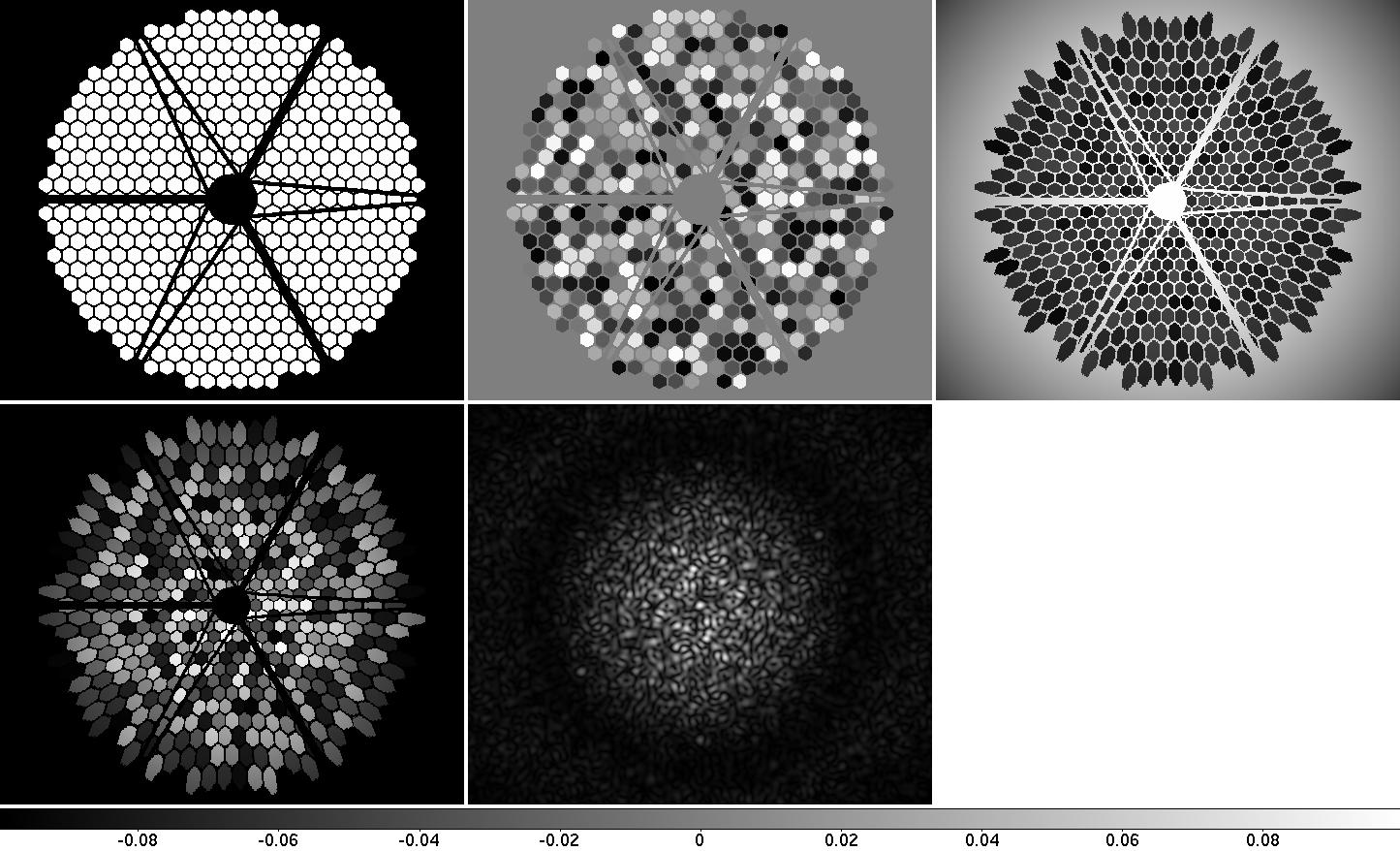
The TMT pupil is used here as an example of a highly segmented pupil. The TMT coronagraph design #1 given in this link is adopted, and offers, in the absence of cophasing errors or other wavefront aberrations, perfect rejection for an on-axis point source. The coronagraph is based on the PIAACMC technique, and offers full throughput and small sub-λ/D inner working angle (IWA). Figure 2.1 shows the result of the simulation with a cophasing error e=0.1 rad (corresponding to a 0.0577 rad RMS phase error).
If the TMT pupil were unobstructed and fully paved, it would consist of 491 segments. The expected contrast level in this example, according to equation (1), is therefore 0.05772/491 = 6.78e-6. As shown in figure 2.2, this prediction is in good agreement with the numerically computed PSF radially averaged contrast.
| |
Fig 2.1: Effect of cophasing error on coronagraph performance. The entrance pupil amplitude (top left) and phase (top center) chosen in this example correspond to the TMT pupil with segment phases following the uniform probability distribution from -0.1 rad to +0.1 rad. The coronagraph output pupil (top right) shows that most of the light is diffracted outside the pupil, but a small amount of light remains in the pupil due to cophasing errors. After applying the Lyot mask (bottom left), the contribution of each segment to the coronagraphic leak is seen to be propotional to the square of the segment phase error. The final on-axis PSF (bottom center) shows that the speckle halo follows the envelop defined by the diffraction pattern of a single segment.
|
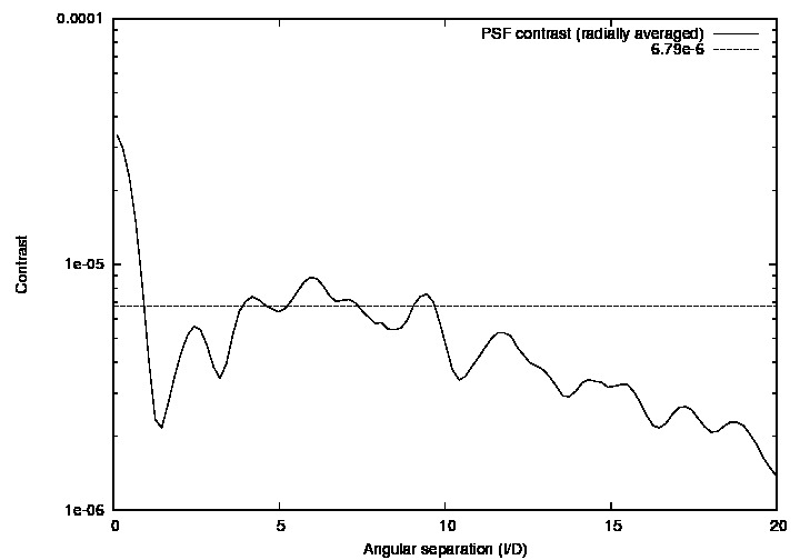 |
Fig 2.2: Contrast as a function of angular separation for the example shown in figure 2.1. The contrast level predicted by equation (2) for the inner region of the PSF is shown as a horizontal line.
|
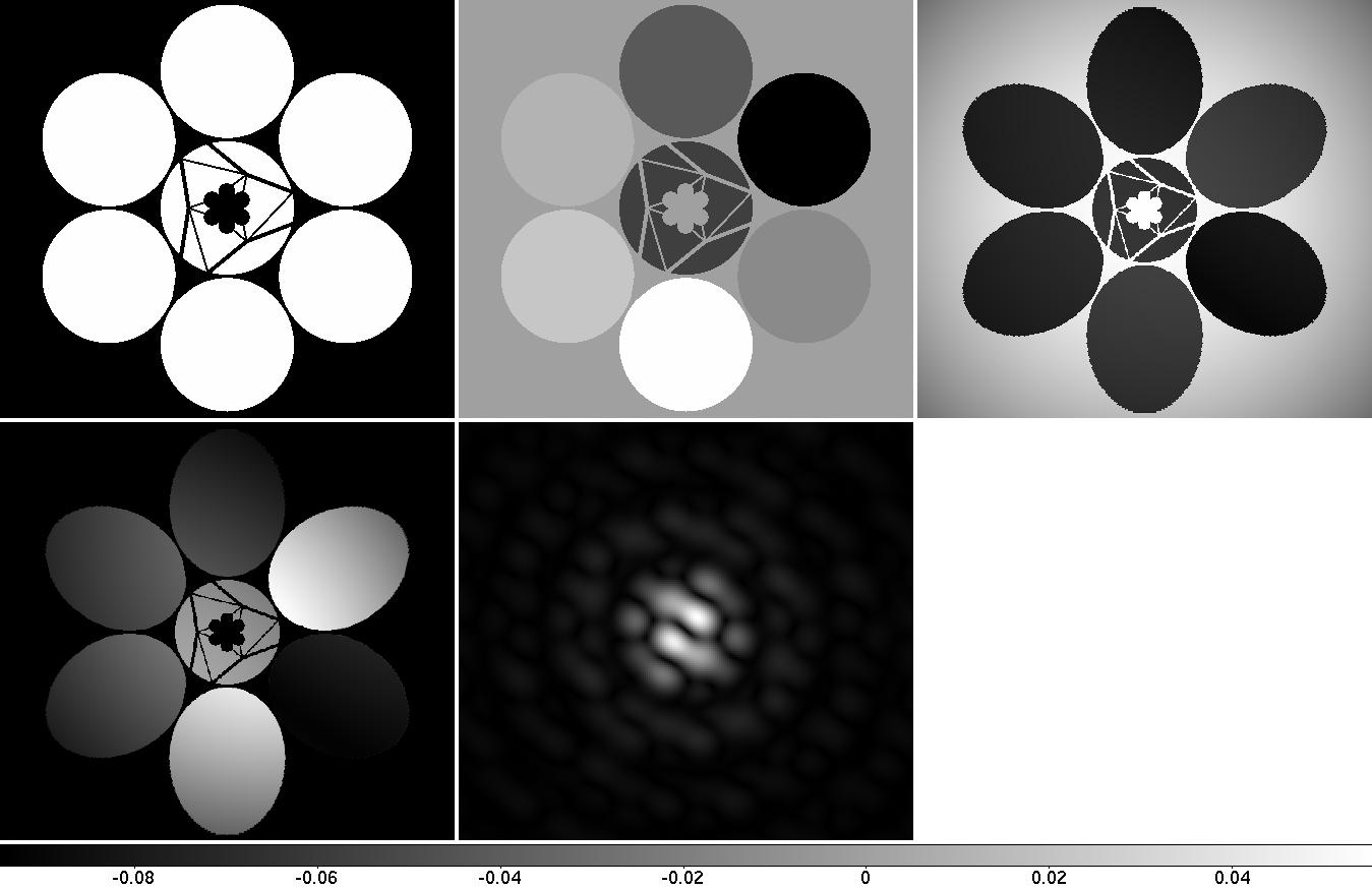 |
Fig 2.3: Effect of cophasing error on coronagraph performance for the GMT pupil. See figure 2.1 caption for details.
|
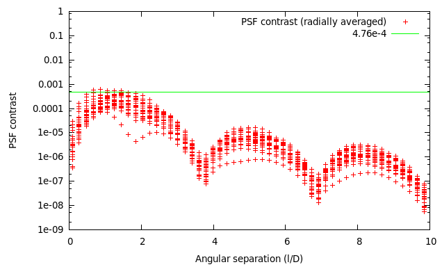 |
Fig 2.4: Contrast as a function of angular separation for the example shown in figure 2.3. The contrast level predicted by equation (2) for the inner region of the PSF is shown as a horizontal line. 24 realizations of cophasing errors are shown. eps file |
| σφ(t) = 1/sqrt(Nph seg) = 2 / ( d sqrt(π 9.7e10 2.512-m t δλ) ) = 1/2760 (1/d) sqrt(1/(t δλ)) 2.512(mV-10)/2 [rad] | (3) |
|---|
Once the contrast requirement is set, equations (2) and (3) can be used to derive a stability requirement by first establishing the cophasing error requirement with equation (2), and then associating a corresponding timescale from equation (3). For example, if the contrast goal requires cophasing error to be no more than 1nm, and if measurement of a 1nm cophasing error requires 5 sec, then the requirement is that the segment phases must not drift by more than 1nm over a 5 sec period. In reality, active control of segment phases cannot be performed at the sampling frequency, and a factor 10 is adopted here to account for this: the stability timescale adopted here is chosen to be 10 times the value given by equation (3). The choice for the value of this factor is somewhat arbitrary, as its exact value is a function of the control loop details and the temporal power spectral density of the segment phase errors. In favorable cases where the segment phase error is a simple function of time (such as a drift at a constant rate, or a single frequency oscillation), the control loop can predict the input disturbance and the factor can become equal of less than 1. For simplicity, only the unpredictible part of cophasing errors is considered here, and it is assumed that any predictible component (such as a drift at a constat rate) can be efficiently removed.
The cophasing requirement obtained from equation (2) is:
| dφ = sqrt( N x Contrast) | (4) |
|---|
It is important to note that the cophasing error required to meet a given contrast level is independant of telescope diameter. With a larger number of segments, the cophasing error can be larger, as the corresponding speckle halo is spread over a larger area in the focal plane.
| t = 1.31e-6 x 2.512mV-10 / ( Contrast x D2 x δλ ) | (5) |
|---|
Examples are given in table 1, assuming that the wavefront sensing is done at λ=550nm with an effective spectral bandwidth δλ=0.1μm.
| Telescope diameter (D) & λ | Number of Segments (N) | Contrast | Target | Cophasing requirement | Stability timescale |
|---|---|---|---|---|---|
| Ground-based telescope | |||||
| 10 m, 1.6 μm | 36 | 1e-6 | mV=8 | 1.5 nm | 21 ms |
| 30 m, 1.6 μm | 10 | 1e-6 | mV=8 | 0.8 nm | 2.3 ms |
| 30 m, 1.6 μm | 1000 | 1e-6 | mV=8 | 8.1 nm | 2.3 ms |
| Space-based telescope | |||||
| 4 m, 0.55 μm | 10 | 1e-10 | mV=8 | 2.8 pm | 22 mn |
| 8 m, 0.55 μm | 10 | 1e-10 | mV=8 | 2.8 pm | 5.4 mn |
| 8 m, 0.55 μm | 100 | 1e-10 | mV=8 | 8.7 pm | 5.4 mn |
In segmented telescopes, the relationship between segment cophasing error and PSF contrast at small angular separation (within the diffraction limit of individual segments) is simple and independent of coronagraph design. Requirements on the allowable cophasing errors and, for an actively controlled system, the open loop stability necessary to meet this requirements, can then be derived.
One key result of this paper is that, with the assumption that cophasing errors are uncorrelated between segments, the allowable cophasing error grows with the number of segments. Correlated cophasing errors (created for example by large scale flexures of the structure holding the segments) were not considered in this study, and could invalidate this conclusion. While we have only considered wavefront control systems using starlight for optical metrology, internal metrology using laser interferometry could be required if the temporal bandwidth required for active control of cophasing errors cannot be achieved with starlight.
The conclusions of this study also apply to segment tip-tilt errors, as the physical origin of unwanted diffracted light in the PSF is phase steps at the interfaces between segments. These phase steps can be produced either by cophasing or tip-tilt errors on the segments. At angular separations larger than the diffraction limit of a single segment, the coronagraph design may be tuned to mitigate sensitivity to segment cophasing errors, and no universal relationship between image contrast and cophasing error exists.