Wavefront Sensing theory

A WFS is an optical device which converts phase aberrations into intensity modulations. All WFSs interferometrically combine different parts of the beam to produce intensity signals. How these interferences are performed is a function of the WFS architecture (Shack-Hartman, Curvature, Pyramid...). For example, in a Shack-Hartman WFS, interferences are performed within each subaperture by image formation.

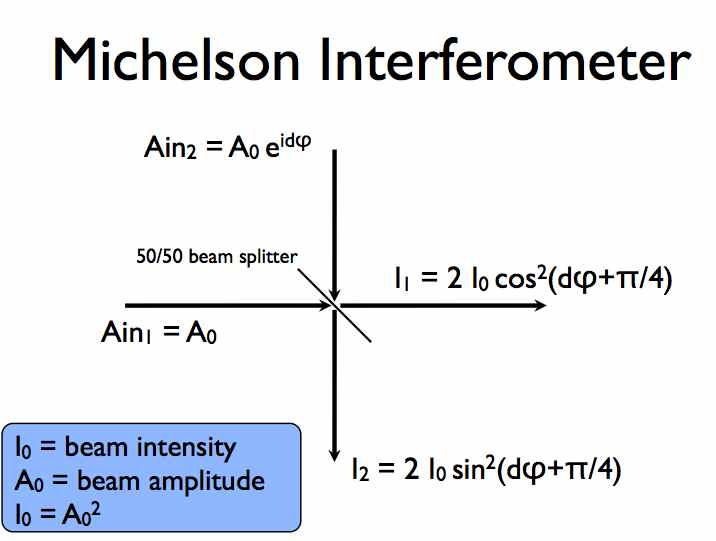The simplest WFS is a two-beam interferometer (Michelson interferometer), where two beams of intensity I₀ each are interferometrically combined and give two output beams.

The intensity of the two outputs encodes the phase difference dφ between the two beams (note that the reference for the phase difference dφ is arbitrary, and has been chosen here such that if dφ=0, the two ouputs have the same intensity):

I₁ = 2 I₀ cos²(dφ+π/4)	(1.1)

I₂ = 2 I₀ sin²(dφ+π/4)	(1.2)

This simple concept can be generalized to all WFSs, with more numerous interferometric combinations which are also not usually simple pairwise intereferences. This generalized representation of WFSs is quite powerful, as it allows an algebraic representation of WFSs in the form of a linear complex amplitude operator.

1.2. Coherence in WFSs

Equations (1.1) and (1.2) given above assume full coherence between the two beams. This is the ideal case, where the intensity modulation will be optimal and the phase reconstruction will therefore require few photons. There are unfortunately several "coherence killers" which will degrade the strength of the WFS. It is important to understand these effects, as they are very often the key limitation in WFS efficiency:

Time coherence. In equations (1.1) and (1.2), dφ can vary during the WFS exposure time. The WFS then measures an attenuated intensity signal, averaged over dφ.
Spatial (in the pupil) coherence. If light is combined between two points of the pupil which are widely separated, and the source is spatially extended, dφ varies across the source. The WFS then measures an attenuated intensity signal.
Chromatic coherence. If the WFS is chromatic, the signals I₁ and I₂ are a function of the wavelength.

2. Wavefront sensing sensitivity, linearity and range

The most desirable WFS properties are:

Sensitivity: How efficiently does the WFS use a given number of photons ?
Linearity: How linear is the relationship between the WF and the WFS output signal
Sensing range: How large a wavefront aberration can be measured

Other important properties, not discussed here, include chromaticity, optical complexity, number of required detector pixels, required computing power. I show in this section that it is fundamentally impossible to get all 3 properties at the same time, but it is possible to have two of the properties. For example, linear WFSs with large range will have poor sensitivity, and WFSs with full sensitivity and large range are non-linear.

2.1. Sensitivity

2.1.1. Theoretically ideal sensitivity

If the WFS is measuring a single WF mode (for example, focus), and N photons are available for the measurement, the 1-sigma error E on this mode should be

E = 1/sqrt(N)	(2.1)

where E is in radian RMS on the pupil. This result can be derived numerically from the complex amplitude linear operator representation of WFSs. The method is described in Appendix XX of this paper. When M modes are sensed, the combined 1-sigma wavefront error is therefore (assuming no correlation between the modes):

E = sqrt(M/N)	(2.2)

2.1.2. Example: Tip-tilt sensing

2.1.3. How to get ideal sensitivity ?

I consider here a single spatial frequency (a phase sine wave across the beam) in the small aberration regime. For simplicity, I also consider a 1-D pupil ranging from x=-1 to x=1. The phase on the pupil is

pha(x) = sin(xCPA/(2π))	(2.3)

where CPA is the cycles per aperture (= spatial frequency) of the sine wave phase aberration considered.

2.1.4. Low coherence WFSs

2.1.5. High Coherence WFSs

2.3. Linearity

Since any WFS can be represented as a linear operator in complex amplitude, the output intensities in a WFS are the square modulus of a linear combination of the input beam phase. The square modulus operator can be linearized over a small range ( the well known (1+x)^2 ~ 1 + 2x for x<1 ). A WFS will therefore be linear if and only if the measured intensities result from the interferometric combination of phase elements with less than ~1 radian phase offset . For example, as shown in the figure below, equations (1.1) and (1.2) show that for dφ < 1 rad:

dφ ~ (I₂-I₁)/(2*I₀)	(2.4)

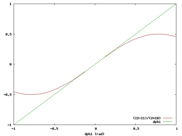
From this linearity condition, we can see that any wavefront sensor will be linear if the wavefront aberrations are small.
A WFS can still be linear for large WF errors if it only performs interferences between points which are spatially close to each other in the pupil, as these points will stay within 1 rad of each other even in the presence of strong large scale aberrations. Examples include a high order SH WFS or a conventional curvature WFS with images close to the pupil plane.

2.4. Sensing range

3. Focal Plane WFS

4. Non-linear Curvature WFS

Page content last updated: 27/06/2023 06:35:52 HST
html file generated 27/06/2023 06:34:36 HST