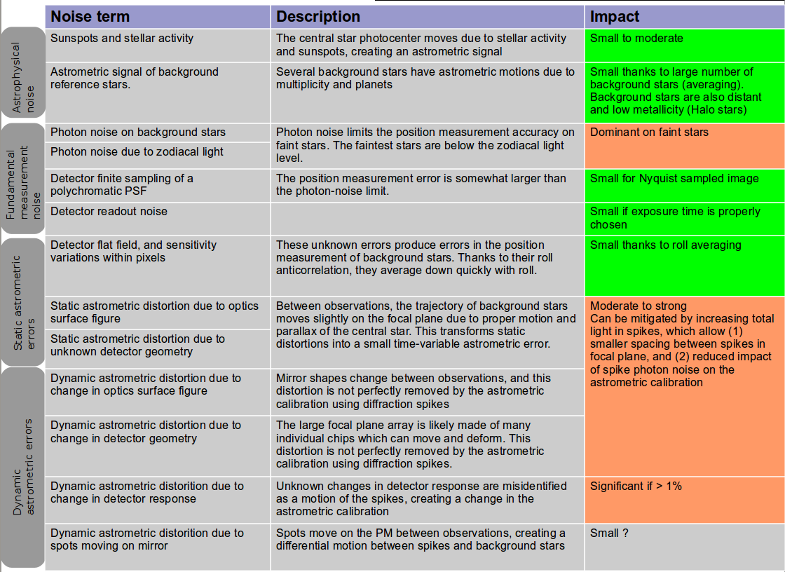
Error budget terms are divided in 4 categories: astrophysical noise, fundamental measurement noise, static astrometric error terms, and dynamic astrometric error terms.
Includes stellar activity on the central star and astrometric wobble of background reference stars.
Measurement noise due to the primary design parameters such as telescope diameter, pixel sampling and wavelength. This would be equal to the total instrument noise in the absence of defects in the detector or optical train. Includes photon noise contribution from background stars and zodi background.
Contribution of all static defects, such as poorly calibrated detector response or manufacturing errors in the optical surfaces. Even perfectly static defects produce astrometric errors, as the trajectories of the background stars on the focal plane are slightly different between observations (proper motion, parallax).
Errors due to changes of the telescope and instrument between observations. Includes variations in the shape of optics surfaces, variations in detector geometry (detector pixels move between observations) and variations in detector sensitivity. Dynamic errors are not fully calibrated by the spikes (spikes have a limited SNR, and do not fully sample the field of view). Dynamic errors can also create errors in the measurement of the spikes positions.
| |
Figure 4-1: Overview of main error budget terms.
[png]
Error budget terms are divided in 4 categories: astrophysical noise, fundamental measurement noise, static astrometric error terms, and dynamic astrometric error terms. |
Figure 4-2 shows that the system simulated differs from the final system (which meets the science requirement). The difference is entirely due to computing limitations:the full scale system image sizes would be 40kx40k pixel (>6 GB per image), too large for the fast and easy computation of the astrometric measurement accuracy necessary for parameter optimization and searches (note that all simulations shown here were performed on a laptop computer, and a more powerful computer could perform the computations on a full scale system).
 |
Figure 4-2: Numerical simulation: parameters.
[png]
Main telescope and instrument parameter values adopted for the numerical simultion. |
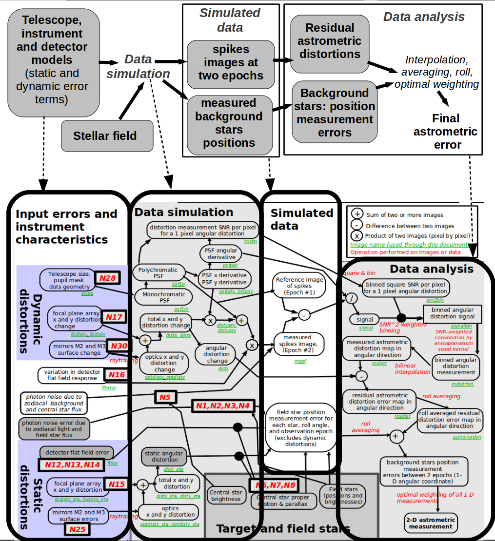 |
Figure 4-2: Numerical simulation overview. [png] Detailed block diagram: [png] List of noise sources (N1 to N30, shown in red on figure): [png] Key steps in the numerical simulation are described in the pdf document. |
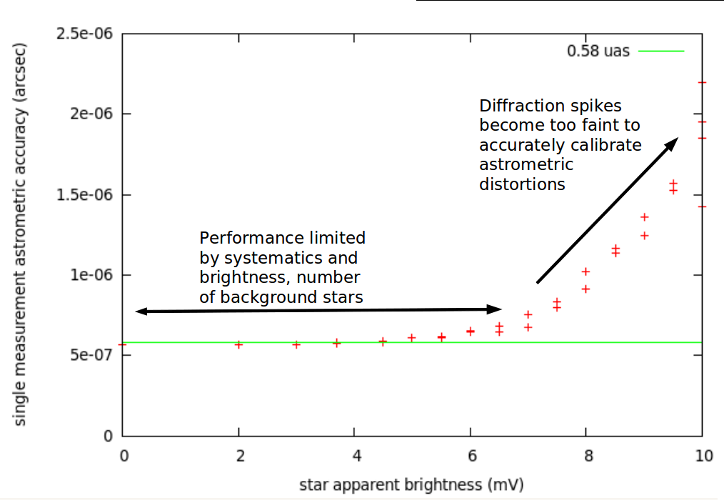 |
Figure 4-3: Single measurement, single axis astrometric measurement accuracy as a function of field of star brightness for the 0.03 sq deg FOV system simulated.
[png]
|
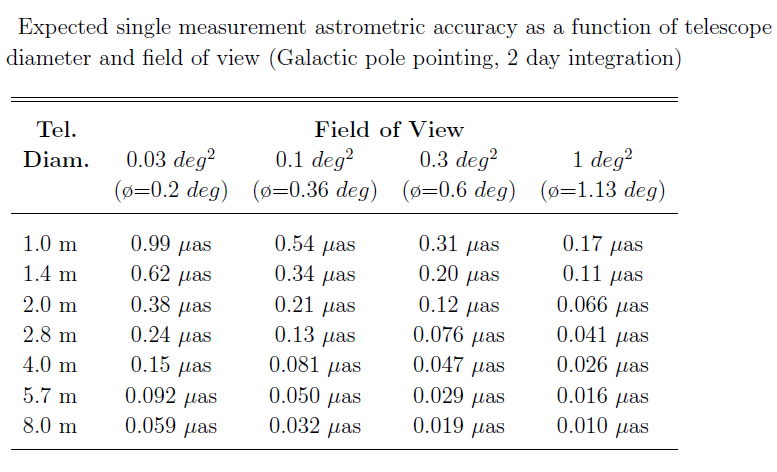 |
Figure 4-4: Single measurement, single axis astrometric measurement accuracy as a function of field of view and telescope diameter.
[png]
|
![[png]](figures/numsimuloverview.png)
![[png]](figures/Noises.png)