This section provides an overview of data acquisition and processing. A more detailed and quantitative analysis in given in Error budget, Simulations.
2. Data acquisition and processing
2.1. What is measured ?
The astrometric signal to be measured is a 2-D translation of the foreground star against a set of fainter background stars used as the astrometric reference. As shown in Figure 2-1, the telescope is pointed on the central star, so the spikes, in principle, do not move between observations, but the background stars move on the detector due to the astrometric motion of the central star (green vector in Figure 2-1). The telescope pointing is essentially dragged by the motion of the foreground star over the course of the mission (several years).
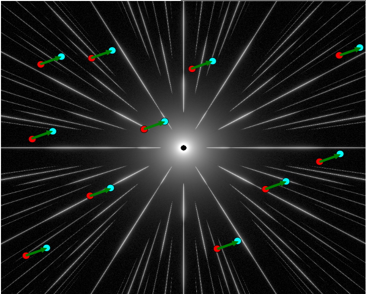 |
Fig 2-1: Measurement principle.
[png]
A set of background stars is imaged in a wide field of view around the central star. The positions of the background stars is shown in this figure in red for the first observation and in blue for the second observation. The green vector (to be measured) is the astrometric motion of the central star between the 2 observations. The motion of the background stars has been greatly exagerated in this figure to illustrate the measurement.
|
The green vector in Figure 2-1 is what the instrument measures as a function of time. This vector is the sum of the foreground star proper motion, the parallax motion and the astrometric signal imprinted by one or several planets. The measurement needs to be repeated at several epochs (typically 10 or more) to unambiguously separate these terms and measure the planet's orbit and mass.
2.2. Distortions
Instrumental astrometric distortions are due to non-ideal optics shapes and detector geometry. While most of the distortions are expected to be static, some are dynamic (variable between observation epochs). Over a fraction of a degree, the instrumental distortions are much larger than the astrometric signature of a planet. As shown in Figure 2-2, the distortions affect both the background stars and the diffraction spikes, so the diffraction spikes can be used to calibrate them.
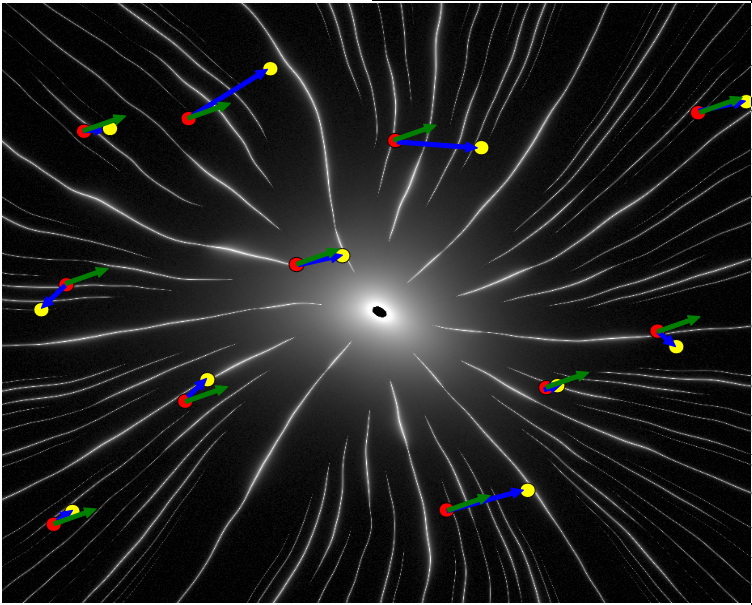 |
Fig 2-2: Effect of astrometric distortions on the image.
[png]
Due to astrometic distortions between the 2 observations, the actual positions measured (yellow) are different from the blue point in Figure 2-1. With a wide field camera, the error is much larger than the signal induced by a planet, which makes the astrometric measurement impossible without distortion calibration. For illustrative purpose, the distortion shown here is 1e6 times larger than expected from high quality optics in the 1.4-m TMA design considered in this study.
|
The measured astrometric motion (blue vectors in Figure 2-2) is the sum of the true astrometric signal (green vectors) and the astrometric distortion induced by changes in optics and detector geometry between the 2 observations. Direct comparison of the spike images between the 2 epochs is used to measure this distortion, which is then subtracted from the measurement to produce a calibrated astrometric measurement.
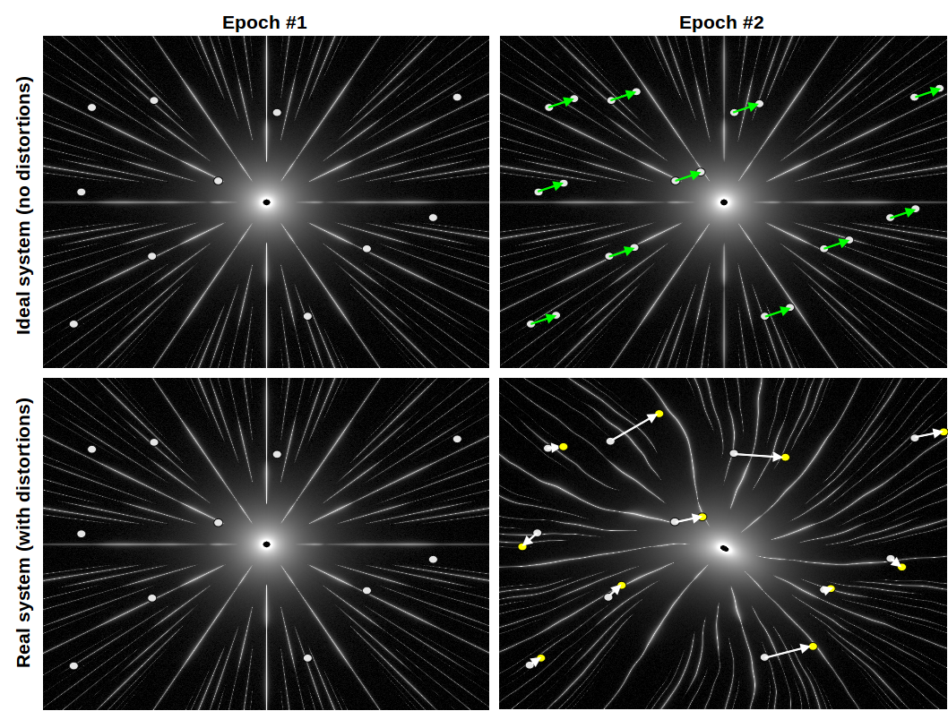 |
Astrometric measurement without (top) and with (bottom) a differential astrometric distortion between observation epochs.
[png]
[ppt]
[eps]
|
2.2. From 1-D measurements to a 2-D astrometric measurement
The calibration of astrometric distortions with the spikes is only accurate in the direction perpendicular to the spikes length: with finite SNR, it is practically impossible to detect a radial motion of the spikes (note: spectral features introduced by a filter could in principle remove this limitation at the expense of throughput).
For a single background star, the high precision measurement is therefore made along the axis perpendicular to the spikes (1-D measurement), as shown by the green vectors in Figure 2-3. The 2-D measurement is obtained by combining all 1-D measurements (large green vector).
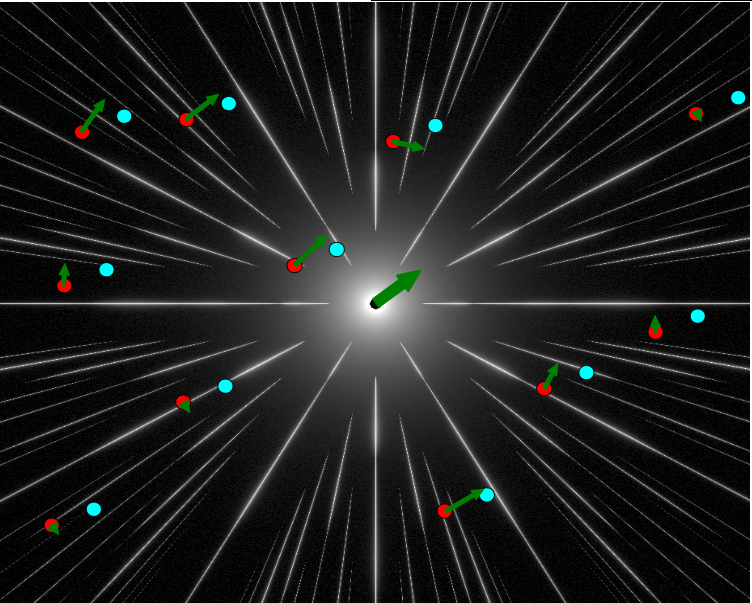 |
Fig 2-3: 1-D astrometric measurement made for each background star (small green vectors), and overall 2-D astrometric measurement (large green vector).
[png]
|
2.3. Telescope roll
2.3.1. Why is a roll needed ?
Detector imperfections can have a large effect on astrometric accuracy. There are two approaches to mitigate this problem:
- Keep the star(s) on nearly the same pixel position between measurements to perform a differential measurement which is insensitive to detector imperfections, or
- Average down detector defects by performing a large number of measurements over different pixels.
In this case, the first approach is not possible: it is not possible to keep background stars on exactly the same pixels of the detector during the measurement timescale (several yr between the first and last measurement).
- (1) The central star's proper motion will drag the background stars at approximately 1 arcsecond per year (30 pixels per year in the example considered) for nearby stars
- (2) The parallax for the coronagraph targets is up to a few tens of arcsecond (a few pixels)
- (3) The aberration of light changes the plate scale by up to 1e-4. For a 0.1 deg field radius (0.1 sq deg) and 40mas pixels, this effect is about 1 pixel at the edge of the field.
While (1) and (2) are pure translations, effect (3) is a stretch. It would conceptually be possible to keep the telescope pointing fixed to the background stars and compensate with a tip-tilt mirror in the coronagraph, but the diffraction spikes would then move on the detector.
Since background stars cannot be kept on the same pixels, each measurement of the motion of a background star between two epochs compares PSFs falling on different pixels with different characteristics (pixel sensitivity, size, shape etc..). Many statistically independent measurements are required to average this error term. This averaging is achieved by both combining the position measurements of a large number of background stars and rolling the telescope along the line of sight to move the background stars' PSFs over a large number of pixels. The roll geometry is shown in Figure 2-4.
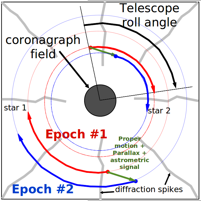 |
Fig 2-4: Position of two background stars on the camera focal plane during telescope roll. Observations at two epochs (colored red and blue) are shown for the two stars.
[png]
|
The telescope roll is very efficient at reducing the contribution of detector errors to the final astrometric measurement. During a single observation (typically a day), the telescope is slowly rolled around the line of sight to move the background PSFs on the focal plane. On a large format detector, a roll angle of a few tens of degrees is large enough to move the PSF by several thousand pixels, and a 1 radian roll will produce about 10000 PSF centroid measurements per star.
2.3.2. Roll Anticorrelation
Unknown flat field errors produce astrometry measurement error: a pixel which is more sensitive than assumed will "attract" the measured position while pixels less sensitive that assumed will "push away" the measured position. Figure 11 shows how this measurement error (red arrows) evolves as the PSF drifts across the detector during telescope roll. The error can be decomposed into a radial component (along the direction to the central star) and a longitudinal component. When integrated over time, the residual error is almost entirely radial, as the longitudinal error when the PSF approaches the defective pixel is compensated by the opposite error when the PSF drifts away from the defective pixel. The telescope roll can therefore almost entirely remove flat field induced errors along the axis where the astrometric measurement is performed.
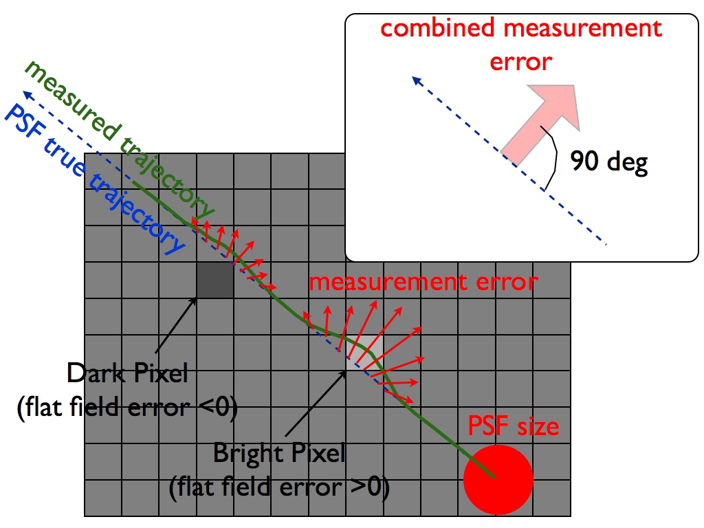 |
Fig 2-5: Effect of flat field errors between pixels on the astrometric measurement of a PSF moving in a straight line.
[jpg]
The true PSF trajectory (blue) differs from the measured PSF position (green curve) due to the presence of "bright" and "dark" pixels. When compensated for the telescope roll, the combined measurement error is perpendicular to the PSF motion: there is no error along the direction of the PSF motion.
|
The discussion above assumes sensitivity differences between pixels, but is also valid for other differences between pixels, such as a pixel with a peculiar color "preferences", or a pixel with a "dead corner". The key advantage of the roll is that it transforms detector defect induced astrometric errors into a time-variable error which is strongly anticorrelated on both sides of the defect. These errors therefore disappear in the averaged measurement (this is much better than a decorrelated error which slowly decreases as sqrt(T)).
2.4. Data Processing Overview
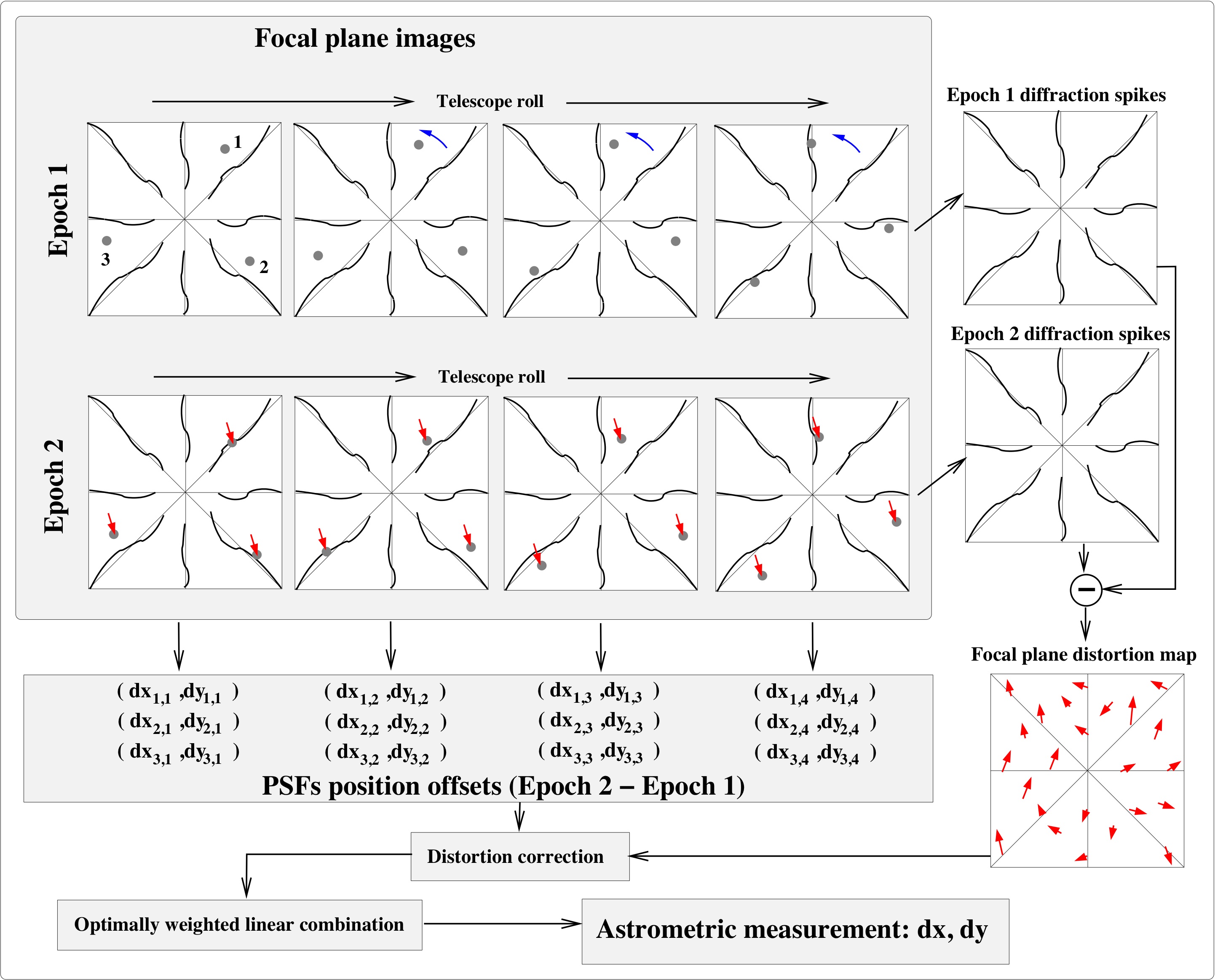 |
Fig 2-6: Data acquisition and data processing overview.
[jpg]
[eps]
|
The data acquired is represented in the top left part of Figure 2-6. The astrometric measurement is performed differentially, between sets of images acquired at 2 epochs. The top row shows 4 images acquired at epoch 1. The telescope is rolled between each image: the diffraction spikes are fixed on the detector but the background stars (grey spots labeled 1, 2 and 3 in the top left image of the figure) rotate around the line of sight. The same sequence of measurements is repeated at epoch 2 (second row). The displacement of the background stars compared to the central star (and the spikes) is shown as red arrows in the epoch 2 images. The background stars are located almost (but not exactly) on the same position on the detector at the two epochs. This configuration is largely immune to uncalibrated/unknown PSF shape, as the PSF is not expected to change sufficiently over a sub-arcsec field to introduce an astrometric error. Maintaining nearly the same PSF positions between epochs also greatly reduced sensitivity to large static distortions (which should also be fully removed by the spike calibration).
The position of the star on the detector is measured by fitting a model of the PSF on a model of the pixel geometry and sensitivity map (including sensitivity variations within the pixels, if known). The position offset (dxi,j,dyi,j), the difference between background star position at two epochs, is measured for each star i in the field for each roll angle position j.
Correction of focal plane distortions
The diffraction spikes are kept at approximately the same position on the detector for all observations, and possible time-variable field distortions are measured by small changes in the shape/location of the spikes. These distortions are only measured along the spikes and a 2-D interpolation is used to build a continuous 2-D map of the distortion change between the 2 epochs. This distortion map is removed from the measurements. The final 2-D astrometric measurement is obtained by combining all 1-D measurements with appropriate weighting coefficients (fainter stars where the photon noise contribution is large are given a smaller weight)
2.5. From images to a 2-D map of angular distortion: algorithm details
We detail here how images of the spikes are compared to produce a distortion map. The discussion here assumes two images I1 and I2 are acquired at different epochs. We note that the two images may themselves be averages of multiple images. They could for example be sigma-clipped averages of images acquired at different roll angles to remove background stars and only leave the spikes.
The following procedure assumes that the intensity on each pixel is a linear function of distortion. This is only true if the distortion is smaller than ~0.5 lambda/D (which should be the case for a space mission). If this is not the case, some rough re-centering (or remapping) to align the images to a fraction of a pixel needs to be done before this algorithm can be executed.
- STEP 1: Construct a reference image Iref by averaging the two images: Iref = (I1 + I2)/2
- STEP 2: Compute the angular derivative dIref/dthetapix = r dIref/dtheta of the reference image: this measures how intensity changes for each pixel for an angular motion locally equal to one pixel. This map can also be computed from the derivatives of the reference image in x and y:
dIref/dthetapix = r dIref/dtheta = -sin(theta) dIref/dx + cos(theta) dIref/dy
- STEP 3: Estimate, for each pixel of the image, the radial displacement of the spikes between the two epochs. This is done by computing (I2-I1)/(dIref/dthetapix)
- STEP 4: Compute, for each pixel, what is the SNR of the distortion measurement for a one pixel distortion
- STEP 5 (optional - but quite useful to speed up computataions): bin the measured raw distortion and SNR map to a smaller image size. The measured distortion is binned with SNR2 weighting to produce the binned version of the measured distortion.
- STEP 6: Interpolate the noisy measured distortion map into a smooth 2-D distortion map. The result from step 4 (or 5) is a pixel-by-pixel estimate of the distortion. On most pixels, especially the pixels between the spikes, this measurement is meaningless as there is no signal and the estimate is dominated by noise. Some interpolation is therefore required to combine, for each point of the image, the nearby measurements with be highest SNR.
- STEP 6.1: Select pixels with a high SNR (the 10%)